九州大学応用力学研究所 Reports　No.154（Mar. 2018）

全文

(1)ISSN 1345-5664. 九州大学応用力学研究所所報. No. 154 March 2018.

(2) CONTENTS. 3D Numerical analysis of free surface shape in the floating zone (FZ) silicon growth with induction coil By Xue-Feng HAN, Xin LIU, Satoshi NAKANO,Hirofumi HARADA , Yoshiji MIYAMURA and Koichi KAKIMOTO.........................................................................................................1 On the Application of Cross Bispectrum and Cross Bicoherence By Sanae–I. ITOH, Kimitaka ITOH, Yoshihiko NAGASHIMA and Yusuke KOSUGA….......6 Inverse Estimate of Air Pollutant Emissions with Multi-wavelength Mie-Raman Lidar Observations By Keiya YUMIMOTO, Itsushi UNO, Tomoaki, NISHIZAWA, Zhe WANG, Yukari HARA, Atsushi, SHIMIZU, Nobuo SUGIMOTO and Ichiro MATSUI......……..............................18.

(3) Reports of Research Institute for Applied Mechanics, Kyushu University No.154 (1-5) March 2018. 3D Numerical analysis of free surface shape in the floating zone (FZ) silicon growth with induction coil Xue-Feng HAN*1, Xin LIU*1, Satoshi NAKANO*1, Hirofumi HARADA*1 , Yoshiji MIYAMURA*1 and Koichi KAKIMOTO*1 E-mail of corresponding author: han0459@riam.kyushu-u.ac.jp (Received January 26, 2018). Abstract The floating zone process includes a molten silicon zone between the feed rod of poly crystalline silicon above and single crystalline silicon below. The molten silicon zone is maintained by the high frequency induction coil. The stability of the molten silicon zone is crucial for the growth process. The shape of the molten silicon zone is determined by the surface tension force, electromagnetic force and hydrostatic pressure in the melt. Since the induction coil is not symmetric, 3D numerical model has been developed for asymmetric shape of the free surface. In this model, 3D Young-Laplacian equations have been solving using volume of fluid (VOF) model. The effect of electromagnetic force has been considered. Concentric and eccentric cases have been calculated. The calculation results are validated by the experimental results. Keywords : Floating zone, Silicon, Computational fluid dynamics. 1. Introduction FZ silicon is widely used for power devices for its high purity and low concentration of oxygen. The molten silicon is heated by the induction coil in the FZ crystal growth. The needle-eye inductor is developed for single crystal growth with large diameters. The high surface tension force and electromagnetic force stabilize the molten silicon above the single crystal silicon. The shape of free surface has an effect on the heat transfer and fluid flow. During the crystal growth in the experiment, the crystal and induction coil block the view of the full free surface. In particular, the interface shape is difficult to predict if the diameter of crystal is large. The heat is generated by high-frequency currents at thin layer adjacent to the free surface. The currents and magnetic field also generate an inward electromagnetic force at the free surface. The layer is small enough that the force is assumed to be applied at the free surface. The high surface tension, strong electromagnetic force and hydrostatic pressure determine the shape of the free surface.. *1 Research Institute for Applied Mechanics, Kyushu Univ.. Coreill et al. presented the calculation for the shape of the free surface 40 years ago [1]. They suggested a 2D model to solve Young-Laplace equation by cylindrical coordinate system. Wünscher used this method to calculate the free surface with the effect of EM pressure and compared to the experimental results [2]. However, 2D axis-symmetric calculation results could not explain the asymmetric effect in the experiment. In the industrial process, to improve the homogeneity of distribution of impurities, the eccentric growth mode is employed [3]. In the eccentric growth mode, the feed rod and crystal are not co-axial. The free surface should not be assumed as 2D axis–symmetric for eccentric growth. Additionally, there is a main slit in the induction coil. The asymmetric shape of inductor induces asymmetric electromagnetic field at the free surface. The force applied at the free surface is also not symmetric. Therefore, in this study, 3D numerical model is developed to calculate the shape of free surface. VOF model is used to solve 3D Young-Laplace equations. The inductor is also included in the model to obtain the 3D electromagnetic field. The 3D electromagnetic force has been coupled with the shape of free surface. The contact angle of silicon is considered when the boudanry conditions of internal triple point (ITP) and external triple point (ETP) are corrected. The calculation results.

(4) 2. Han et al.: 3D Numerical analysis of free surface shape in the floating zone (FZ) silicon growth with induction coil. have been validated by comparison experimental results from Wünscher [2].. 2.. with. the. Computation method. In this study, as shown in Fig. 1, we have constructed a simulation model for FZ silicon crystals with a diameter of 50 mm (2 inch), taking into account the argon gas and the silicon melt. The size of the model is according to the experiment from Wünscher et al. [2]. The positions of ETP, melting front and solid-liquid interface are fixed in the model. A 3D finite volume mesh is constructed using the mesh tool (snappyHexMesh [4]). The hexahedral mesh is used because the hexahedral mesh shows better stability than the tetrahedral mesh in OpenFOAM. Silicon melt and gases are considered as incompressible fluids to improve computational stability.. Here, 𝜌1 and 𝜌2 are the density of argon gas and silicon melt, respectively. The compressibility of fluid is ignored. The divergence of velocity in the volume is zero: ∇∙𝑼 =0 Combining the continuity equation, we can derive the following equations: ∇∙𝑼=−. −. The model includes gas and melt. To calculate the interface between tow fluids, VOF model in OpenFOAM was used coupling with continuity equation (1) and Navier–Stokes equations (2): 𝜕𝜌 + 𝛻 ∙ (𝜌𝑼) = 0 𝜕𝑡. (1). 𝜕𝜌𝑼 + 𝛻 ∙ (𝜌𝑼𝑼) − 𝛻 ∙ 𝜏 = −𝛻𝑝 + 𝑆 𝜕𝑡. (2). Here ρ, U, 𝑡, 𝜏, p, and S are density, velocity vector, time, stress tensor, pressure, and source term, respectively. Surface tension force 𝐹𝜎 and gravity 𝜌𝑔 are included in the source term: 𝑆 = 𝐹𝜎 + 𝜌𝑔 = 𝐶𝑘 ∇𝑎 + 𝜌𝑔. (3). where 𝑎 is liquid fraction, 𝐶𝑘 is surface tension coefficient. Surface tension force can be calculated by 𝐶𝑘 ∇𝑎. The density is given by the following equation: 𝜌 = 𝑎𝜌1 + (1 − 𝑎)𝜌2. (4). 1 𝐷𝜌 𝜌 𝐷𝑡. (6). 1 𝐷𝜌 1 𝐷(𝑎(𝜌1 − 𝜌2 ) + 𝜌2 ) = − 𝜌 𝐷𝑡 𝜌 𝐷𝑡 (7) =−. 𝜌1 − 𝜌2 𝐷𝑎 =0 𝜌 𝐷𝑡. The volume fraction can be given in the equation as follows: 𝐷𝑎 𝐷𝑡. Fig.1 Concentric model of FZ for 50 mm (2 inch) diameter single crystal silicon. (red part is inductor). (5). =. 𝜕𝑎 𝜕𝑡. + ∇ ∙ (𝑎𝑼) = 0. (8). Electromagnetic force at thin layer pushes the shape of the free surface inwardly. So the calculation of high-frequency electromagnetic field is essential to investigate the shape of free surface. Due to the asymmetric distribution of the current density in the inductor, three-dimensional electromagnetic field needs to be considered. Since the electromagnetic field is caused by the induced current, three-dimensional inductor mesh is also constructed. The current density distribution in the inductor is calculated. For high-frequency electromagnetic field, the heat power is adjusted by changing the voltage between the electrodes. Therefore, it is considered that the electric potential difference between the electrodes is known. Under the electric potential boundary conditions, the electric field can be calculated: 𝑬 = −𝑔𝑟𝑎𝑑(𝜑). (9). here 𝑬 is electric field, and 𝜑 is electric potential. From Ohm’s law, the current density 𝑱 can be calculated from electric fields: 𝑱 = 𝜎𝑬. (10). where 𝜎 is conductivity of inductor. Magnetic vector potential 𝑨 can be derived by the following equation: ∇2 𝑨 = −𝜇𝑱. (11).

(5) Reports of Research Institute for Applied Mechanics, Kyushu University No.154 March 2018. 3. 𝜇 is the permeability for the copper. The magnetic field can be calculated by the curl of magnetic vector potential 𝑨: 𝑩=∇ × 𝑨. (12). Under the effect of magnetic field and current at the free surface, the electromagnetic force forms at the free surface. The force is given by the equation: 𝑭𝑬𝑴 = 𝑗 × 𝑩. (13). Fig.2 Silicon melt fraction (red part) and gas fraction (blue part) distribution: (a) initial condition; (b) final result after 1 s transient calculation. where 𝑭𝑬𝑴 is electromagnetic force volume density. If the magnetic field is known, the electromagnetic force can be solved by using the following equation: 𝑭𝑬𝑴 = −. 1 𝑔𝑟𝑎𝑑(𝑩2 ) 2𝜇. (14). Since the skin layer is so thin that the EM force 𝑭𝑬𝑴 is imposed at the interface between the argon gas and the silicon melt. Finally, the source term in the Navier-Stokes equation is revised as following form: 𝑆 = 𝑭𝝈 + 𝜌𝑔 + 𝑭𝑬𝑴. 3.. (15). Results and Discussion. We performed transient calculations using the model described above. In the first case, we assume that the feed rod and the crystal are coaxial. And both the feed rods and the crystals are stationary (Fig. 1). In the initial stage, the space between the feed rod and the crystal is filled with silicon melt (Fig. 2a). Since single crystal can not support too much melt, excessive melt drops due to gravity. This phenomenon has also been experimentally studied [5], especially when the crystal diameter is large. After transient calculation, the melt is stable (Fig. 2b), showing a stable interface between the gas and the melt. A stable free surface starts with ETP and ends with ITP. ETP is determined by the shape of the crystal, its diameter is 50 mm. However, ITP is calculated by VOF model that takes into account the contact angle between the melt and the feed rod. In Fig. 2b, at the top of the model, the rest of the melt does not flow down due to the contact angle boundary conditions. The amount of remaining melt is exactly the upper limit that the crystal can support. The interface coordinates are extracted to form a three-dimensional free surface, as shown in Fig. 3. The shape is symmetric despite the deviations at the periphery. Due to the surface tension of silicon and the inward force from electromagnetic field, the shape of the free surface is stable even if the diameter of the FZ silicon is. Fig.3 3D interface shape in concentric mode: (a) front view; (b) perspective view large. Electromagnetic pressure distribution is determined by the magnetic field distribution, mainly by the geometric design of the inductor coil. The geometry of the inductor in this study is according to the experimental results obtained by Wunscher et al. [6]. There are three side slits and one main slit in the inductor (Fig. 4a). This design makes electromagnetic heating more uniform. The electric potential difference between the electrodes is 1 volt. The potential distribution is shown in Fig. 4a. The potential drops evenly from the positive electrode to the negative electrode. Fig. 4b shows the current density vector distribution. The maximum current density occurs at the tip of the side slit and at the contact part between the electrodes and the inductor. This phenomenon is described in previous calculations due to the concentration of current [6].. Fig.4 (a) Electric potential distribution of inductor under 1 V condition; (b) current density vector distribution in the inductor Since the current density distribution inside the heater has been calculated above, the magnetic field distribution can be calculated. The results shown in Fig. 5a confirm that the magnetic vector is in the same direction as the current in the inductor. Since the furnace wall is electrically conductive, we assume that the value of the magnetic vector is zero at the furnace wall, which.

(6) 4. Han et al.: 3D Numerical analysis of free surface shape in the floating zone (FZ) silicon growth with induction coil. is considered to be the boundary of the computational domain. So the magnetic vector potential drops from the inductor to the furnace wall. Fig. 5b shows the magnetic field around the heater. The magnetic vector rotates around the inductor. Under applied current conditions, the maximum value is 2 Tesla. The purpose of the side slit is to distribute the magnetic field more widely.. three-dimensional calculations show a higher position than the experimental results. Though VOF model and 2D assumption do not consider the rotation effect and temperature, they are both credible to predict the shape of the interface by solving Young-Laplace equations. Because the free surface is three-dimensional, three-dimensional electromagnetic field calculations are also applied to the model. In order to consider the effect of the electromagnetic field on the free surface, electromagnetic pressure is incorporated into the VOF model. We assume that the frequency of the electromagnetic field is a constant value of 3 MHz. Fig. 6b shows the comparison of the calculated results of 2D and 3D free surfaces and experimental results. Compared with Fig. 6a, the electromagnetic field calculation results fit better with the experimental results because the magnetic pressure significantly pushes the free surface to the inside. This also indicates that under high-frequency magnetic field, the silicon melt is more stable.. Fig.6 (a) Magnetic vector potential distribution; (b) magnetic field distribution Because the three-dimensional calculation method is different from the two-dimensional calculation method, it is necessary to discuss the validation of this method by comparing the simulation results with the existed experimental data. Fig. 6 shows the comparison of experimental and calculation results. The experiment, conducted by Wunscher et al. [2], used a camera system to capture the image during the 2-inch FZ silicon crystal growth [6]. In Fig. 6a, the white dashed line shows the result of a two-dimensional assumption without the electromagnetic force calculated by Wunscher et al. [6]. The red line is the 3D calculation from the VOF model without electromagnetic force. It can be seen that the 3D results of the VOF model are in good agreement with the 2D results of the previous study. Since the inductor block the view of ITP, the calculation line is longer than the experimental free surface. Without the influence of electromagnetic force, the two-dimensional and. Fig.5 Comparison of free surface shape between 3D calculation results, 2D calculation results, and experimental results [2]: (a) no electromagnetic force in the calculation; (b) with electromagnetic force in the calculation.

(7) Reports of Research Institute for Applied Mechanics, Kyushu University No.154 March 2018. Fig.7 Eccentric model of FZ for 50 mm (2 inch) diameter single crystal silicon. (red part is inductor) As shown in Figure 7, we also built an eccentric model to analyze the free surface. In this model, the relative positions of the feed rod and crystal are shifted by 5 mm. The other initial and boundary conditions are the same as the previous concentric calculation. In this new calculation, we assume that the ETP position remains unchanged even though the position of the feed rod and the inductor has changed. Through transient calculation results, a three-dimensional asymmetric free surface is obtained (Fig. 8). As can be seen from the side view of the free surface, the shape of the curve varies greatly in different directions, which can lead to different heating power distributions. The location of ITP also changed. In the actual growth process, if the inductor has changed, ETP and solid-liquid interface should be changed. This effect will be discussed in future research work. The successful calculation of three-dimensional asymmetric freeform surface will provide a good foundation for the future research on asymmetric induction heating.. process of FZ grown single crystal silicon was obtained. In order to study the influence of the electromagnetic field, the current distribution of the inductor and the distribution of the electromagnetic field are calculated in three-dimension. The 3D electromagnetic results show a similar distribution with the previous study. It is confirmed that the magnetic pressure drives the free surface inward. By introducing the electromagnetic field into the VOF model, the 3D calculation results are in good agreement with the previous 2D and experimental results. We have successfully calculated the shape of free surface under both concentric and eccentric growth condition. The realization of an accurate free surface helps to increase the accuracy of study on the heat transfer, mass transfer and crystal quality in the future.. Acknowledgment This work was partly supported by the New Energy and Industrial Technology Development Organization (NEDO) under the Ministry of Economy, Trade and Industry (METI).. References 1). 2). 3). Fig.8 3D interface shape in eccentric mode: (a) front view; (b) perspective view. 4.. Summary. By developing a combined model of transient VOF model and electromagnetic field model based on finite volume method, a three-dimensional free surface in the. 5. 4) 5) 6). S. Coriell, M. Cordes, Theory of molten zone shape and stability, Journal of Crystal Growth, 42 466-472, 1977 M. Wünscher, A. Lüdge, H. Riemann, Growth angle and melt meniscus of the RF-heated floating zone in silicon crystal growth, Journal of Crystal Growth, 314, 43-47, 2011 W. Dietze, W. Keller, A. Mühlbauer, Crystal Growth, Properties and Applications, in, Springer, Berlin, 1981. https://openfoam.org/release/2-3-0/snappyhexmesh. D.-I.R. Menzel, Growth Conditions for Large Diameter FZ Si Single Crystals, PhD thesis. M. Wünscher, R. Menzel, H. Riemann, A. Lüdge, Combined 3D and 2.5D modeling of the floating zone process with Comsol Multiphysics, Journal of Crystal Growth, 385, 100-105, 2014..

(8) 九州大学応用力学研究所所報第 154 号 ( 6 - 17 ) 2018 年 3 月. Cross Bispectrum と Cross Bicoherence の活用について伊藤早苗*1,2 伊藤公孝*2,3 永島芳彦*1,2 小菅佑輔*1,2 (2018年1月31日受理). On the Application of Cross Bispectrum and Cross Bicoherence Sanae –I. ITOH, Kimitaka ITOH, Yoshihiko NAGASHIMA and Yusuke KOSUGA E-mail of corresponding author: s-iitoh@riam.kyushu-u.ac.jp Abstract Bispectrum and bicoherence analysis is a powerful method to analyze nonlinear interaction of turbulent plasmas. In this note, we explain the difference of the bispectrum and bicoherence analysis and possible research that can be pursued with these methods. Basic concept is explained by using several examples from previous successes brought by bicoherence and bispectrum analysis, such as drift wave-zonal flow interaction. Open questions are discussed that can be challenged by these methods. Problems such as spatial transport of fluctuation energy (i.e. turbulence spreading), momentum transport by the triplet correlation, and so on, are treated. Bispectrum and bicoherence analysis can be utilized to expand the forefront of plasma turbulence research. Keywords: plasma turbulence, nonlinear coupling, bicoherence analysis. 1.. 解析手法が標準化し，収束等の理解も深まり、bicoherence. 緒言. 解析を活用して更に広い問題にチャレンジ出来るようになっ. 磁場閉じ込めプラズマでは、ドリフト周波数帯領域の低周波揺動が重要な役割を果たしている. 1)。特に、線形分散. ている。さらに、入門的な解説も 21, 22)などに見られる。 bicoherence 解析では、同一の物理量を対象に求める. 、磁. auto-bicoherence と、異なる物理量を組み合わせて解析する. 化高温プラズマの乱流や構造形成を理解するためには、非. cross-bicoherence がある。その両者を活用する事で、更に研. 線形相互作用の理論及び実験による研究が重要である。非. 究が進むと期待出来る。例えば、帯状流の場合、密度とポ. 線形相互作用の観測に Bicoherence 解析が活用されている。. テンシャル揺動の auto-bicoherence と cross-bicoherence に. を大きく変えてしまうほど非線形相互作用が強いので. 2). 3-9) などが見られる。実測された. は違いがある事が予想され、その差違も検証される事で理. bispectrum の値と乱流揺動の非線形結合度の定量比較な. 解が更に深まっている。微視的揺動のみならず、揺動のエ. ども行われ. ンベロープと言う新たな観測量を抽出し、それを対象にした. 初期の適用例には 10). 、非線形結合の定量解析が可能になってきた。. 近年、帯状流 11)のように、線形安定である一方ドリフト波から. cross-bicoherence によって、密度揺動には見えないとされて. 非線形励起される揺動の重要性が認識されるにつれ、. いた帯状流の観測にも成功している. bispectrum 解析は実際の実験研究で広く応用されるように. spectroscopy という新たな方法 23)の典型例である。. 14). 。これは parametric. 9,12-17)。その結果、帯状流や帯状磁場、ストリーマー. 近年の観測では、密度やポテンシャルと言ったスカラー. などの励起機構が実験的に検証されるなど、重要な発見が. 場の量のみならず、速度場揺動などベクトル場の揺動も観. もたらされた. 12, 15, 16, 18)。これらの応用例を含め、プラズマ研. 測され、ベクトル場とスカラー場の非線形結合も興味を集め. 究の強力な方法として広く活用されている。プラズマの構造. ている。多くの種類の物理量の探索において、それで何が. 19, 20)にまとめて紹. 解明できるのかという明確な問題意識とともに、どんな高次. 介されている。最近は、bicoherence 解析はルーチンになり、. 統計解析が必要かという展望を持つことが望まれる。その観. なった. 形成の物理への応用の俯瞰的な結果が. *1 *2 *3. 九州大学応用力学研究所九州大学極限プラズマ研究連携センター中部大学総合工学研究所. 点から、密度やポテンシャル揺動、速度揺動などの crossbispectrum や cross-bicoherence を解析する事により広がり.

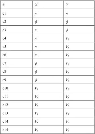
(9) 九州大学応用力学研究所所報第 154 号 2018 年 3 月うる研究の可能性が俯瞰的に論じられている. 24)。ここでは、. 今後研究の具体的実験観測を容易にし、我が国において. 7. Angelo mode25-36), また、帯状流. 11)、ストリーマー18)、などが. 揺動として励起される可能性があるとする。. 広く活用を図ることを目的として、和文報告としてそうしたテーマを紹介する。この研究論文では、密度やポテンシャル揺動、速度揺動. 2.2. 二次相関. などの cross-bispectrum や cross-bicoherence を解析する事. <X, Y>（<…>は同一位置での長時間平均）は標準的に. により広がる研究を説明する。なお、bispectrum 解析という. 解析されている。今は、同一点の物理量を対象にしている. 言い方や、bicoherence 解析という言い方がよくなされてい. ので、時間フーリエ分解した. る。ここでは、両者の区別を活かして説明を進める。Cross-. 𝑋(𝑓)𝑌(𝑓)∗. 及び auto-bicoherence 解析は規格化された値を使う。あるプロセス（モードの組み合わせ、など）に着目し、その非線形. で議論する。組み合わせを Table.１に示す。. 結合度を（他の多分観測されていない寄与と比較して）定量化する際に威力を発揮する。その一方で、cross-bispectrum. ここで auto-correlation (c1, c2, c10, c11, c12)は揺動強度として標準的に解析される。スカラー量を見ると、<nn>と<>の比は、ドリフト波を検. では絶対値も含めた物理量の相関を論じる。物理量の強度の絶対値や、空間的輸送束などを解析する際に重要となる。. (1). 定する中心的手法である。適切に規格化して、. それぞれに特徴ある意味を持つので、cross-coherence 解析. n n n0 n0. や cross-bispectrum 解析を駆使することで、物理量の非線形結合や輸送解析を実験定量的に解析できる。. . e e Te Te. (2). の関係は、ドリフト波の検定の基礎に使われる。ここで n0 は時間平均された密度である。. 2.. Model. 2.1. 対象の説明. 磁化プラズマを考える。議論の明確化のため、 slab plasma を考え、磁場を z 方向に取る。（Fig.1 参照。）drift 速度や、磁場方向速度を示しておく。局所的な座標として(x,y) を導入し、x が r に, y がに対応するものとする。. Fig.1 Magnetized inhomogeneous plasmas with two driving sources. Shown are radial gradients of density (pressure) and flows along the magnetic field. In the local coordinate, z is in the direction of the magnetic field, x is in the direction of inhomogeneity, and y corresponds to the poloidal direction. また、揺動は準静電的揺動として、密度(n)やポテンシャル揺動()、速度揺動(V)が測られているものとする。ここで. Table 1: Combinations of second order correlation #. X. Y. c1. n. n. c2. . . c3. n. . c4. n. Vx. c5. n. Vy. c6. n. Vz. c7. . Vx. c8. . Vy. c9. . Vz. c10. Vx. Vx. c11. Vy. Vy. c12. Vz. Vz. c13. Vx. Vy. c14. Vx. Vz. c15. Vy. Vz. は、時間スケールをドリフト周波数およびそれよりゆっくりした変動に限る。温度揺動は重要な物理量であるが、計測例が極めて限られているので、ここでは論じない。このような条件で、不安定揺動としては、drift mode1), D’. Cross correlation の中では、c3 は密度とポテンシャルの位相差を求めるためにルーチンとして解析されている。ドリフト.

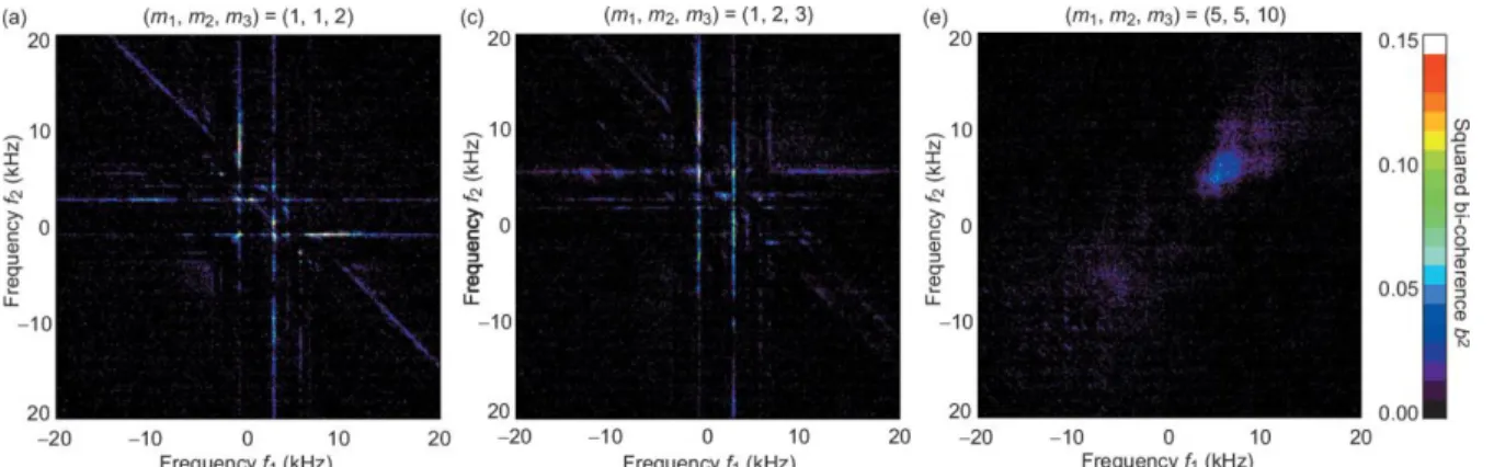
(10) 伊藤・伊藤・永島・小菅：Cross Bispectrum と Cross Bicoherence の活用について. 8 波の場合は. 2. n e  (1  i ) n0 Te. (3). がよく知られている。例えば、抵抗性ドリフト波の場合. 31)には、. 2.  e   n   V         (1   s2 k2 ) n   c  T   e   0  s . 2. (8). と表現されている。. 位相差は. 最近の研究例では、２次相関より得られる揺動強度がモードの判別に応用されている。ドリフト波に比し、D'Angelo. . *e   2 z. k Dz. mode では平行速度揺動が相対的に大きくなる。この特徴を、 (4). c1, c12 を利用して、ドリフト波の場合 n n V V  z z n0 n0 cs cs. で与えられる。*e はドリフト周波数、 Dz は電子の磁場方向拡散係数である。位相差は波の励起の因果関係や密度勾配の緩和に伴う有限の粒子束を表すものと理解されている。. となるのに対し、D'Angelo mode の場合には. 実験データ解析にて評価もされている。. V V n n  z z n0 n0 cs cs. D’Angelo mode の場合は n e  n0 Te. (9). (5). (10). と表すことができる。実際のデータ解析を通じて、ドリフト波と D'Angelo モードが異なる半径や周波数空間に共存すること. となる。断熱応答に近く、これは、D’Angelo mode は平行速. が報告されている 32,36)。. 度シアによって駆動されるためである。D’Angelo mode は平行速度揺動に特徴があり、平行速度を緩和する。粒子束による分布の緩和がエネルギー源ではないので、ドリフト波と. 0.1. は異なり、勾配方向の粒子束を作るとは限らない。. 150 (a) squared bicoherence (SN98390). そして、ドリフト波と D’Angelo mode が混在している場合、相関は. k z2 Dz . 50. 50. (7). frequency 2 [kHz]. Angelo モードからの寄与 31)は. V . 100. (6). となる。ここで、位相差はドリフト波の場合と同様であり、D’ cs k z  s k y Vz   cs2 k z2. 0.0 0.5 1.0 phase (rad/(2π)) 150 (a) biphase (SN98390). 100. frequency 2 [kHz]. n e  (1  i D  iV ) n0 Te. 0.05 0.00 significance levels=0.005. 0. 0. -50. -50. -100. -100. である。cs はイオン音速、s は電子温度で評価されたイオンラーマー半径である。D’Angelo mode が不安定な場合である。ドリフト波は密度勾配を緩和させる位相関係を持つ一方で、D’Angelo mode は密度勾配をピークさせる（密度勾. -150 0. 配に抗う粒子束を生み出す）位相関係を持つことが報告されている。また、ベクトルとスカラー量の混合では、nVx (c4)は乱流輸送流束として解析されて来た。一方で、類似の量 nVy (c5), nVz (c6)は揺動に伴う運動量密度に対応するが、余り実験で評価されてはいないようである。ところで、c4 と c7 などは、ドリフト波では n ~ なのであるが、c4 で残るのは１次の微少量であり、c7 では面平均をとると打ち消される。一方、ベクトル量の相関については VxVy (c13), VxVz (c14), VyVz (c15)がしばしば Reynolds stress の評価に使われる。最後に、c1, c2, c10 + c11 + c12 は揺動強度に結びつく。揺動強度は、ドリフト波を記述するモデルでしばしば. 40 80 120 frequency 1 [kHz]. -150 0. 40 80 120 frequency 1 [kHz]. Fig.2 Examples of bispectral analysis for drift wavezonal flow turbulence in JFT-2M tokamak. (a) Bicoherence and (b) biphase analyses of floating potential fluctuation. The figures are quoted from Y. Nagashima, et al., PPCF 45 S1 (2006), and their layout is changed.. 3.. Bispectrum and cross bispectrum. 3.1. Third order correlation.

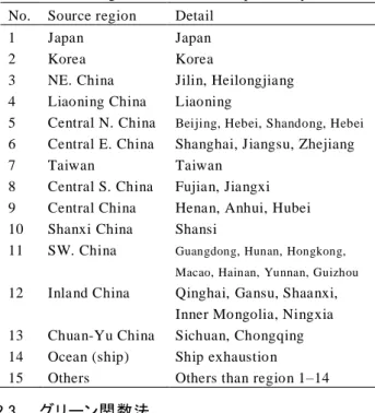
(11) 九州大学応用力学研究所所報第 154 号 2018 年 3 月. 9. Fig.3 Example of bicoherence analysis with the mode number matched. Here the 2D Fourier spectrum in frequency and the poloidal mode number is evaluated from the azimuthal probe array (64 channels). Bioherence in frequency is evaluated for the data with mode number matched, m3=m1+m2. Three different cases are shown, with (m1, m2, m3) = (1,1,2), (1,2,3), and (5,5,10). The figure is quoted from 38). 三次相関<X, Y, Z>（<…>は同一位置での長時間平均）. b12. . . Vz. b13. n. . Vz. b14. n. Vx. Vx. b15. n. Vy. Vy. いる。（例を Fig.2 に示す。）非線形結合は、波数空間のマッ. b16. n. Vz. Vz. チング条件も満たさなければならない。そこで、波数空間の. b17. n. Vx. Vy. b18. n. Vx. Vz. を拘束条件として周波数上で bispectrum 解析を行うことで、. b19. n. Vy. Vz. 波数と周波数の双方のマッチング条件を満たす非線形相. b20. . Vx. Vx. b21. . Vy. Vy. b22. . Vz. Vz. b23. . Vx. Vy. b24. . Vx. Vz. は、非線形機構の研究のため着目され研究されている。多くの適用例では、周波数分解して、 𝑋(𝑓1 )𝑌(𝑓2 )𝑍(𝑓1 + 𝑓2 )∗. (11). を bispectrum として解析し、実験結果を対象に応用されて. フーリエスペクトルを扱う解析もしばしば行われている 18, 37)。さらに踏み込んだ解析. 38)では、波数空間のマッチング条件. 関を求めている。例を Fig.3 に示す。これらを念頭に置いた上で、本稿では、周波数空間での bispectrum 解析を念頭に置いて議論する。 Table 2: Combinations of triplet correlation #. X. Y. Z. b1. n. n. n. b25. . Vy. Vz. b2. . . . b26. Vx. Vx. Vx. b3. n. n. . b27. Vx. Vy. Vy. b4. n. . . b28. Vx. Vz. Vz. b5. n. n. Vx. b29. Vx. Vx. Vy. b6. . . Vx. b30. Vx. Vx. Vz. b7. n. . Vx. b31. Vx. Vy. Vz. b8. n. n. Vy. b32. Vy. Vy. Vy. b9. . . Vy. b33. Vy. Vz. Vz. b10. n. . Vy. b34. Vy. Vy. Vz. b11. n. n. Vz. b35. Vz. Vz. Vz.

(12) 10. 伊藤・伊藤・永島・小菅：Cross Bispectrum と Cross Bicoherence の活用について. スカラー場の量とベクトル場の量による３次相関を Table 2 ラーとベクトル量の混交の bispectrum、b26~b35 がベクトル. n2. n2. に示す。b1~b4 がスカラー量の bispectrum, b5~b25 が、スカ量の bispectrum である。. Time No Flux. Vx. Vx. Finite Flux Time. Time. Time. Fig.5 Spatial flux of fluctuation energy (represented by density fluctuation). Finite spatial flux results when the time evolution of fluctuation energy and radial velocity fluctuation are in phase. 帯状流とドリフト波の密度揺動に対する現れ方の違いを利用して両者の非線形性の違いや、ランダムな乱流揺動スペクトルが一様に帯状流によって変調されているというような発見に結びついている。更に、b1, b2, b3, b4 の違いを観察する事で、ドリフト波と帯状流の定性的な違いを描き出している（Fig.4）。それは、帯状流の変動が密度では微少である一方、電場（ポテンシャル）に集中して現れるからである。帯状流の周波数を f とする。n の周波数が f になる組み合わせでは、顕著な bispectrum のピークが見えない。一方、の周波数が f になる組み合わせでは、顕著な bispectrum のピークが現れる。密度揺動そのものではなく、高周波密度揺動のエンベロープの時系列から周波数 f の成分を抜き出せば、エンベロー Fig.4: Analysis of low frequency fluctuation with floating potential and ion saturation current. Combination of floating potential, (a) auto-power of the floating potential, (b) auto-power of the ion saturation current, and (c) auto-power of the envelope of the ion saturation current, (d) squared cross-coherence between the floating potential and ion saturation current, (e) squared cross-coherence between the floating potential and the envelope of the ion saturation current, and (f) cross-phase between the floating potential and the envelope of the ion saturation current. In (e), significant coherence between the envelope and floating potential at zonal flow frequency (~10 kHz) is observed, indicating the envelope of the ion saturation current has information of zonal flows. The figure is quoted from Ref. 14).. プには帯状流が刻印されているので、{n のエンベロープ, n, n}という組み合わせからも、帯状流と微視的ドリフト波の非線形結合を観測する事が出来る。一方、E×B ドリフトによる揺動電場は通常時間変動がイオンサイクロトロン周波数よりも極めて低いという近似の元で計算されている。一部のプラズマでは、電場振動の時間微分から評価される分極ドリフトの効果が無視できなくなる可能性がある。分極ドリフトの効果は例えば長谷川-三間方程式の導出などで既に導入されている一方、散逸性ドリフト波の様に径方向輸送を伴う系では密度揺動とポロイダル電場揺動の積の統計平均から、静電乱流中のポロイダル電流源として、存在しうる可能性があり、プラズマ中の電流の実測といった新規の研究に結び付く可能性がある。. 3.2. Scalar quantity. スカラー量の bispectrum は帯状流の研究に適用され、有効性を実証した. 8,9,12-14)。帯状流のドリフト波による励起の問. 題ではポテンシャル同士及びポテンシャルと密度を組み合わせたクロスバイスペクトルのような解析が広く行われている。. 3.3. スカラーとベクトル量混交の cross-bispectrum. 3.3.1 揺動強度の空間移動揺動強度が空間移動するような場合が実際に起きており、.

(13) 九州大学応用力学研究所所報第 154 号 2018 年 3 月. 11. 研究が進んでいる。そのような過程を研究するためには、ベ. の２次相関が一粒子あたりのストレスとして、また、乱流によ. クトル量を含む bispectrum が重要になる。輸送現象を研究. る磁場方向の流れの駆動については. するためには、スカラーとベクトル量混交の cross-bispectrum. 𝑉𝑥 𝑉𝑧. は重要な役割りを果たしている。 Drift 波の揺動強度のうち密度変動が持つ成分は 𝑛𝑛. (17). が一粒子あたりのストレスとして解析されている。しかし、 (12). Reynolds stress は 𝑛𝑉𝑥 𝑉𝑦. である。すると. 𝑛𝑉𝑥 𝑉𝑧 𝑉𝑥 𝑛𝑛. (13). (18). 𝑛𝑉𝑦 𝑉𝑧. は、「Drift 波の揺動強度のうち密度変動」が x 方向に移動. の３次相関で定義されている。Cross-bispectrum によって評. する割合を指す。Turbulence spreading で取り扱われる物理. 価されるべきものである 46-51)。. 量である. 39,40)。Figure. 5 に示すように、揺動強度（密度で見. たもの）が時間変動しているとする。同時に Vx も変動してい. まず、プラズマのポロイダル回転励起（径電場駆動）に関係する成分については. る。それらの変動が同期していると、平均として、揺動強度. ⟨𝑛𝑉𝑥 𝑉𝑦 ⟩と𝑛0 ⟨𝑉𝑥 𝑉𝑦 ⟩. が x-方向に移動している事になる。この寄与を求めると、 𝑛(𝑓1 )𝑛(𝑓2 )𝑉𝑥 (𝑓1 + 𝑓2 )∗. (14). という cross-bispectrum を求める必要がある。. (19). の差違について、実験的に検証が行われるレベルになっている 50)。これまでの実験では、ポロイダル方向の渦の伸長に着目した結果、ポロイダル速度揺動と径方向速度揺動の位. ところで、乱流強度の（背景揺動による）空間移送は、乱. 相関係に特に着目し、後者の項が解析されてきた。一方、. 流強度を決める重要な要素であると考えられている。たとえ. 実験データとしては密度揺動も同時に計測している場合が. ば、理論的には、乱流強度 I の空間流束は（局所的なモデ. ほとんどであり、三体相関項を解析することは十分可能な環. ルの範囲で）-D grad I +V I と評価される（しばしば拡散型の. 境が整っている。. 校が重要と見なされている）。その結果、乱流強度は d I   L I   NL I   modI  DI dt. (15). のようなバランス方程式を満たすと考えられている。右辺の第一項は線形励起、第二項は非線形安定化項（ただし、 DC 径電場の空間一次微分に起因する安定化効果. 41）を含. む）、第三項は帯状流との結合効果、第４項が乱流強度の（背景揺動による）空間移送に基づく非線形安定化（励起）効果を示す. 42)。この局所化が適切か否かの問題は措くとし. て、その範囲においても、第４項は、他の３項と比較して、無視出来ない働きをするとされている。実際、理論やシミュレーションを通じて、乱流フロントの伝搬や安定領域の侵食などが報告されている. 43) 。フロントが伝搬することを示唆する. 実験も報告されている. 44,45). 。また、直線プラズマでも、密度. 勾配が強い線形不安定な領域以外でもスペクトルの広がりが観測されている. 36)。cross-bispectrum. Fig.6 Observation of momentum flux. (a) Result on PANTA32). The r is the radial direction and z is the direction of the magnetic field. (b) Result on TORPEX49). The z is the vertical direction and  is the toroidal direction. In both cases, the triplet term (green for (a) and red for (b)) is finite and can be dominant in some cases. 一方、プラズマの磁力線方向の運動励起に関係する成分については（Fig.6）、. を求めることによって、. ⟨𝑛𝑉𝑥 𝑉𝑧 ⟩と𝑛0 ⟨𝑉𝑥 𝑉𝑧 ⟩. 新たな検証が可能になる。. の差違の研究が始まっている. (20). 32,51)。理論的にも、プラズマの. トロイダル回転の variety を理解する上での鍵であると指摘さ. 3.3.2 Reynolds Stress Reynolds stress の重要性は近年理論的／実験的に確認. れている. 46)。２次相関に焦点を当てた残留応力などの効果. されている。通常、乱流によるプラズマのポロイダル回転励. に加え、３次相関を考えることで乱流運動量の空間移送の. 起（径電場駆動）に関係しては. 効果（Turbulence momentum spreading）を取り入れることが. 𝑉𝑥 𝑉𝑦. 可能となる。周辺領域のトロイダル流と炉心領域でのトロイダ (16).

(14) 12. 伊藤・伊藤・永島・小菅：Cross Bispectrum と Cross Bicoherence の活用について. ル流の結合を生み出す効果も指摘されている. 51)。実験的に. 検証が行われる日も近い。例えば、DIII-D トカマクではパラレルレイノルズ応力について３体相関項を含む検証がなされている 52)。複数のレイノルズ応力や粒子束などの輸送量の同時解析は、密度勾配や速度勾配など複数の不均一性（自由エネルギー源）が共存するなかで起きる乱流の理解にとって重要になる。近年、「強相関乱流」という考え方が提案され、プラズマ乱流研究の枠組みが拡張されている. 53)。物性物理学. 分野では「強相関物質」の研究が展開しており、強磁性、強誘電性、等の共存など、複数の巨視的場の自発的発生（交差相関）が熱平衡状態で議論されている。プラズマ乱流に. Fig.8: Development of zonal flows and helical flow pattern by D’Angelo modes34). The bicoherence of vector quantity Vz and scalar quantity , VzVz, can be important for analyzing the process.. おける交差相関も重要であり、巨視場の生成・競合・消滅、トポロジー変化（散逸と対称性の変化）さらに、対称性の破れや対称性の変換などの機構にふかく関与しているものと. 3.3.3 Reynolds Stress （補足）もう一つの組み合わせ. 考えられている。Figure 7 に説明されるように流れと圧力の. 𝑛𝑉𝑦 𝑉𝑧. 勾配が共存する状況は実験室や宇宙のプラズマで広く観察され、２章に説明された drift wave と D’Angelo mode など. については、それに基づく力. がそこで問題となる揺動の例である。半径方向の密度（圧力）. d nVyVz. 勾配と磁力線方向流の勾配を持つプラズマの構造形成機. dy. 構を Fig.7 に概説する。ドリフト波と帯状流の励起・抑制の相互作用が起きることはよく知られている. 11)。それに加え、D’. (21). と. d nVyVz dz. (22). は磁気面平均すると消えるとの発想から、重要視されていな. Angelo mode を介在として密度や軸方向速度の勾配が変化. いものと思われる。しかし、L-H 遷移が起きる場合、ポロイダ. していく。片方の緩和と他方の急峻化が起きることも可能で. ルショックが生まれる事が理論的に指摘され、計算例も示さ. あり、周回方向の速度駆動と、磁力線方向の駆動が転換す. れている事から. ることも可能である。自然界の多様な構造形成機構を反映. ダルショックなど磁気面上で局在した非線形構造の重要性. している。複数種の不安定性や構造形成機構を含む系を. が見いだされる可能性もある。磁気面上で局在した非線形. 念頭に、most probable structure や、交差相関の理論構造. 構造が生まれる過程では、. 54-58)、今後動的観測精度が高まると、ポロイ. （非線形緩和の多様性）や競合する散逸率の定式化などの. d nVyVz. 理論研究が行われている。あわせて、多種の揺動の共存に. dy. 関し観測結果（ Fig.8 ）も得られ始めており. 32,33) 、 cross-. bicoherence 解析を用いて、相互の非線形結合についても実験観測が試みられている。. と. d nVyVz dz. のような、磁気面上で不均一な値を持つ力が、機能を発揮している可能性もある。Cross-bispectrum が重要な値になる可能性がある。(磁気面平均した輸送量だけではなく、輸送量の磁気面の上不均一性も理論的に重要性が指摘されている。例えば Stringer’s spin-up 機構 57, 58)や、揺動の上下非対称性から生まれるトロイダル流構造 59)などについても近年研究が蓄積されており、揺動の不均一性についての実験観測も報告が見られている 60, 61)。こうした過程の実験検証では、新たな corss-bispectrum も活用されるであろう。). 3.3.4 n との差 b5 から b13 までには、 n とが現れている。ドリフト波の場 Fig.7: Structural formation in plasmas with radial gradients of density (pressure) and parallel velocity. In addition to the excitation and suppression of drift waves and zonal flows, D’Angelo modes can drive relaxation and steepening of parallel velocity profile and density profile.. 合は、近似的に n ~ なので、 b5, b6, b7 b8, b9, b10 b11, b12, 13 の性質は近いとされている。しかし、ドリフト波が準モードの.

(15) 九州大学応用力学研究所所報第 154 号 2018 年 3 月. 13. 場合には線形励起に係わるボルツマン関係を常に満たすと. 空間方向の揺動運動エネルギーのフラックスが重要となるこ. は限らない。線形励起されたドリフト波乱流が空間に展開し. とが報告されている(Fig. 9)。. ているか、もしくは Turbulence spreading の様に乱流が広が. ドリフト波の場合では、x-方向の揺動速度と y-方向の揺動速. る場合を cross- bicoherence 解析を異なる空間点で実施比. 度はほぼ等しく. 較することにより、励起機構の差別化の実験検証に結び付. 𝑉𝑥 𝑉𝑥 ~𝑉𝑦 𝑉𝑦. く可能性がある。. (24). である一方、z-方向の揺動速度は相対的に小さく. 3.3.5 ベクトル場が生み出す帯状流. 𝑉𝑥 𝑉𝑥 ~𝑉𝑦 𝑉𝑦 ≫ 𝑉𝑧 𝑉𝑧. ドリフト波と帯状流の結合の検定にスカラー量の. (25). bispectrum が威力を発揮した（ 3.2 章）。その一方で、. となっている。b28 は b26, b27 に比べ重要性が低いと考えら. D'Angelo mode のようなベクトル場が駆動する乱流において. れる。密度との規格化因子を考えて. も帯状流が生成されることが報告. 34,35) され、強相関乱流の. b5, b26, b27. 一例として報告されている（Fig. 9）。こうした結合を検証する. が揺動強度の空間移送を担っている。密度との規格化因子. 際に、. を考えて  n 2  V 2  V     x    y  n0   cs   cs . b22 などが有効となるであろう。また、垂直方向の流れ場（外部駆動等による、２次的な帯状流ではない）が存在し、Kelvin-.    . 2.  Vx  . (26). と表現される。. Helmholtz 不安定性が生じた場合には、. D’Angelo mode の場合には平行方向速度の揺動が無視. b20, b21. できなくなり、空間方向の揺動エネルギー移送は. などの量が鍵となる。.  n  2  V     x  n0   cs . 2.   Vy    c   s. 2.   Vz    c   s.    . 2.  Vx  . (27). となる。空間方向に揺動エネルギーが運ばれる結果、平行速度シアが強くなる不安定領域が空間的に局在していても、 D'Angelo mode の存在領域が広がる可能性がある。このような仮説の検証にも cross-bicoherence 解析が有用となる。. 3.4.2 揺動強度の空間移動(2) 同様の議論は、z-方向の移送現象についても言え、 𝑉𝑧 𝑉𝑥 𝑉𝑥 𝑉𝑧 𝑉𝑦 𝑉𝑦 62) Fig.9: Energy balance of mean field and turbulent ~ field ~~ . The spatial flux of fluctuation energy, T  VrV2 , can play an important role in fluctuation energy balance.. (28). 𝑉𝑧 𝑉𝑧 𝑉𝑧 は、磁力線方向の揺動移送に関係する。今迄余り着目されていない物理量である。しかしながら，スクレイプオフ層 (Scrape-off layer, SOL)における輸送現象では、磁力線に沿った一様性が無いため、磁力線に沿う構造も適切に考える. 3.4 ベクトル量の cross-bispectrum 3.4.1 揺動強度の空間移動(1). 必要がある。SOL の厚みの問題は近年重要性がましており、. 揺動強度が空間移動するような場合には、密度揺動だけ. こうした auto-bispectrum ならびに cross-bispectrum の検討が必要である。. ではなく、揺動の運動エネルギーも移送される。. この場合、ドリフト波揺動の様な圧力勾配揺動では. (15)式に示されるようなバランスを考える上では 𝑉𝑥 𝑉𝑥 𝑉𝑥 𝑉𝑥 𝑉𝑦 𝑉𝑦. Vx  Vz. (23). 𝑉𝑥 𝑉𝑧 𝑉𝑧 が揺動運動の x-方向のエネルギー移送に関連している。実際. 62)、ポロイダル流の運動エネルギーの時間発展を解析し、. (29). であり、径方向の移送が卓越する。その一方で、D'Angelo mode では Vx  V z. (30).

(16) 伊藤・伊藤・永島・小菅：Cross Bispectrum と Cross Bicoherence の活用について. 14. となり、径方向への移送のみならず磁力線方向への移送が重要となる。径方向の移送量  n  2  V     x  n0   cs . 2. 2.   Vy   Vz        c  c    s  s. 2.  Vx  . 束等の理解も深まった研究最前線において、bicoherence 解 (31). 析を活用して更に広い問題にチャレンジ出来る状況を説明した。近年の研究では、密度やポテンシャルと言ったスカラ. や軸方向の移送量  n 2  V     x  n0   cs . この研究論文では、プラズマ乱流揺動の研究において bicoherence 解析がルーチンになり、解析手法が標準化し収. ー場の量のみならず、磁場や速度場揺動などベクトル場の 2. 2.   Vy   Vz        c  c    s  s. 2.  Vz  . (32). を比較することで、D'Angelo モードの特定につながることが期待される。支配的な揺動の特定は輸送特性を考える上で重要であり、今後の検証が待たれる。. 揺動も観測され、ベクトル場とスカラー場の非線形結合も興味を集めている。そのような状況を踏まえ、密度やポテンシャル揺動、速度揺動などの cross-bispectrum や crossbicoherence を解析する事により広がる研究を俯瞰した。 bispectrum, bicoherence が重要であり、それらの実験的活用が勧められる。多くの種類の物理量の探索において、それで何が解明で. 3.4.3 Others. きるのかという明確な問題意識とともに、同時にどんな高次. b31 VxVyVz について、例えば、ポロイダルレイノルズ応力が磁力線方向. 統計解析が必要かという展望を持つことが望まれる。. に移送される量を表す。前項と同様に、磁力線に沿った一. 謝辞. 様性がない系では無視できない可能性がある。. P.H. Diamond 教授、藤澤彰英教授、稲垣滋教授、山田琢. 3.5 計測での新たな留意点最後に、多種のベクトル場やスカラー場の非線形結合を正確に観測するための新たな実験的留意点についても触. 磨博士、小林達哉博士との有益な議論に感謝いたします。本研究の一部は、科研費 (26420852, JP15H02155, JP15K17799, JP16H02442)のサポートを受けました。. れる。異なる種類のベクトル場同士の高次相関を研究するため. 参考文献. にたとえば(28)にあるような cross-bicoherence を求める必要が出てくる。磁力線方向の量と、磁力線に垂直な方向の量との混交した相関を取り扱う。そのためには、観測点での基. 1). York, 1965). 準となる磁力線の方向を正確に観測する必要がある。ドリフト波など、本稿で対象としている揺動は非等方性が極めて. B.B. Kadomtsev, Plasma Turbulence (Academic, New. 2). A. Hasegawa, C. G. Maclennan and Y. Kodama, “Nonlinear behavior and turbulence spectra of drift waves. 強い。磁力線の方向に誤差があると、磁力線方向の量と、磁力線に垂直な方向の量と観測値にクロストークが生じる。. and Rossby waves”, Phys. Fluids, 22, pp.2122-2129,. このクロストークは、高次相関に大きな誤差を齎す事が指摘. (1979) 3). されている 63)。. Ch. P. Ritz, E. J. Powers, T. L. Rhodes, R. D. Bengtson,. この事から、磁場内部の磁場の計測を高精度に実施し、. K. W. Gentle, Hong Lin, P. E. Phillips, A. J. Wootton, D.. 揺動計測や高次相関に齎す誤差を押さえる必要が出てくる。. L. Brower, N. C. Luhmann Jr., W. A. Peebles, P. M.. 通常時期面の観測は、MHD 平衡の再構成という手法で取. Schoch and R. L. Hickok, “Advanced plasma fluctuation. り扱われ、揺動研究とは独立に取り扱われる事が通例であ. analysis techniques and their impact on fusion research (invited)”, Rev. Sci. Instrum. 59, pp.1739-1744, (1988). る。磁気面の決定制度は中型のトカマクで 1cm 程度と議論されている。この誤差は、場合によっては、乱流の高次相関. 4). T. Uckan, J. Harris, and A. J. Wootton, “Experimental. （特に非局所的相関）を議論する上で不満足な結果を齎しう. evidence of three-wave coupling on plasma turbulence”,. る。今後、MHD 平衡較正と、揺動研究を統合して行う事も. Phys. Rev. Lett., 71, pp.3127-3130, (1993). 必要になろう。一つの先駆的試みは、GAM spectroscopy をプラズマの表面磁気面決定に適用した. 64) 。揺動研究の観. C. Hidalgo, E. Sánchez, T. Estrada, B. Brañas, Ch. P. Ritz,. 5). H. Y. W. Tsui, K. Rypdal, Ch. P. Ritz, and A. J. Wootton, “Coherent nonlinear coupling between a long-wavelength. 点から、表面磁気面の検定を論じている。今後は、こうした. mode and small-scale turbulence in the TEXT tokamak”,. 統合的研究を更に展開する事も必要と考えられる。. Phys. Rev. Lett., 70, pp.2565-2568, (1993) 6). 4.. Summary. J. S. Kim, R. J. Fonck, R. D. Durst, E. Fernandez, P. W. Terry, S. F. Paul, and M. C. Zarnstorff, “Measurements of Nonlinear Energy Transfer in Turbulence in the.

(17) 九州大学応用力学研究所所報第 154 号 2018 年 3 月 Tokamak Fusion Test Reactor”, Phys. Rev. Let., 79, pp.841-844, (1997) 7). 8). Zonal Flows in a Toroidal Plasma”, Phys. Rev. Lett., 93, 165002-1-165002-4, (2004). R. A. Moyer, G. R. Tynan, C. Holland, and M. J. Burin,. 16) A. Fujisawa, K. Itoh, A. Shimizu, H. Nakano, S. Ohshima,. “Increased Nonlinear Coupling between Turbulence and. H. Iguchi, K. Matsuoka, S. Okamura, T. Minami, Y.. Low-Frequency Fluctuations at the L−H Transition”,. Yoshimura, K. Nagaoka, K. Ida, K. Toi, C. Takahashi, M.. Phys. Rev. Lett., 87, pp.135001-1-135001-4, (2001). Kojima, S. Nishimura, M. Isobe, C. Suzuki, T. Akiyama,. G H. Xia and M. G. Shats, “Inverse Energy Cascade. Y. Nagashima, S.-I. Itoh, and P. H. Diamond,. Correlated with Turbulent-Structure Generation in. “Experimental Evidence of a Zonal Magnetic Field in a. Toroidal Plasma”, Phys. Rev. Lett., 91, pp.155001-1-. Toroidal Plasma”, Phys. Rev. Lett., 98, pp.165001-1-. 155001-4, (2003) 9). 15. 165001-4, (2007). P. H. Diamond, M. N. Rosenbluth, E. Sanchez, C.. 17) P. Manz, M. Ramisch, U. Stroth, V. Naulin, and B. D.. Hidalgo, B. Van Milligen, T. Estrada, B. Brañas, M.. Scott, “Bispectral experimental estimation of the. Hirsch, H. J. Hartfuss, and B. A. Carreras,“In Search of. nonlinear energy transfer in two-dimensional plasma. the Elusive Zonal Flow Using Cross-Bicoherence. turbulence”,. Analysis”, Phys. Rev. Lett., 84, pp.4842-4845, (2000). pp.035008-1-035008-12, (2008). Plasma. Phys.. Control.. Fusion,. 50,. 10) K. Itoh, Y. Nagashima and S.-I. Itoh, P. H. Diamond, A.. 18) T. Yamada, S. -I. Itoh, T. Maruta, N. Kasuya, Y.. Fujisawa, M. Yagi, and A. Fukuyama, “On the. Nagashima, S. Shinohara, K. Terasaka, M. Yagi, S.. bicoherence analysis of plasma turbulence”, Phys.. Inagaki, Y. Kawai, A. Fujisawa, and K. Itoh, “Anatomy. Plasmas, 12, 102301-1-102301-9, (2005). of plasma turbulence”, Nature Phys. 4, pp.721-725,. 11) P.H. Diamond, S.-I. Itoh, K. Itoh, and T.S. Hahm, “Zonal flows in plasma—a review”, Plasma Phys. Control. Fusion, 47, pp.R35-R161, (2005) 12) Y. Nagashima, K. Hoshino, A. Ejiri, K. Shinohara, Y. Takase, K. Tsuzuki, K. Uehara, H. Kawashima, H.. (2008) 19) S. -I. Itoh, “Plasma Turbulence -Structural Formation, Selection Rule, Dynamic Response and Dynamic Transport”, J. Plasma Fusion Res. 86, pp.334-370, (2010) in Japanese. Ogawa, T. Ido, Y. Kusama, and Y. Miura, “Observation. 20) S.-I. Itoh, S. Inagaki, A. Fujisawa, and K. Itoh,. of Nonlinear Coupling between Small-Poloidal Wave-. “Integrated Research of Dynamic Response and Dynamic. Number Potential Fluctuations and Turbulent Potential. Transport of Plasma Turbulence” J. Plasma Fusion Res.. Fluctuations in Ohmically Heated Plasmas in the JFT-2M Tokamak”, Phys. Rev. Lett., 95, pp.095002-1-095002-4, (2005) 13) Y. Nagashima, S. -I. Itoh, S. Shinohara, M. Fukao, A.. 90, pp.793‐820, (2014) in Japanese 21) T. Yamada and S. Oldenbürger, “Progress of Turbulence Analysis Methods – Multi-Scale Coupling”, J. Plasma Fusion Res., 88, pp.309-314, (2012) in Japanese. Fujisawa, K. Terasaka, Y. Kawai, G. R. Tynan, P. H.. 22) Y. Nagashima and H. Arakawa, “Observation of. Diamond, M. Yagi, S. Inagaki, T. Yamada, and K. Itoh,. Nonlinear Energy Transfer in Plasma Turbulence”, J.. “Observation of the parametric-modulational instability. Plasma Fusion Res., 88, pp.315-321, (2012) in Japanese. between the drift-wave fluctuation and azimuthally. 23) S. –I. Itoh, K. Itoh, M. Sasaki, A. Fujisawa, T. Ido, and Y.. symmetric sheared radial electric field oscillation in a. Nagashima, “Geodesic acoustic mode spectroscopy”,. cylindrical laboratory plasma”, Phys. Plasmas 16,. Plasma Phys. Control. Fusion, 49, L7-L10, (2007). pp.020706-1-020706-4, (2009). 24) Sanae-I.. ITOH,. Kimitaka. ITOH,. Yoshihiko. 14) Y Nagashima, K Itoh, S-I Itoh, A Fujisawa, M Yagi, K. NAGASHIMA and Yusuke KOSUGA, “On the. Hoshino, K Shinohara, A Ejiri, Y Takase, T Ido, “In. Application of Cross Bispectrum and Cross Bicoherence”,. search of zonal flows by using direct density fluctuation. Plasma Fusion Res., 12, pp.1101003-1-1101003-9 (2017). measurements”, Plasma Phys. Control. Fusion, 49,. 25) N. D'Angelo, “Kelvin—Helmholtz Instability in a Fully. pp.1611-1625, (2007) 15) A. Fujisawa, K. Itoh, H. Iguchi, K. Matsuoka, S. Okamura, A. Shimizu, T. Minami, Y. Yoshimura, K. Nagaoka, C.. Ionized Plasma in a Magnetic Field”, Phys. Fluids, 8, pp.1748-1750, (1965) 26) W.E. Amatucci, “Inhomogeneous plasma flows: A. Takahashi, M. Kojima, H. Nakano, S. Ohsima, S.. review. Nishimura, M. Isobe, C. Suzuki, T Akiyama, K. Ida, K.. experiments”, J. Geophys. Res. 104, pp.14481-14503,. of. in. situ. observations. and. laboratory. Toi, S.-I. Itoh, and P. H. Diamond, “Identification of. (1999).

(18) 伊藤・伊藤・永島・小菅：Cross Bispectrum と Cross Bicoherence の活用について. 16. 27) T. Kaneko, H. Tsunoyama, and R. Hatakeyama, “Drift-. Shinohara, N. Kasuya, K. Terasaka, K. Kamataki, H.. Wave Instability Excited by Field-Aligned Ion Flow. Arakawa, M. Yagi, A. Fujisawa, and K. Itoh, “Two-. Velocity Shear in the Absence of Electron Current”, Phys.. dimensional bispectral analysis of drift wave turbulence. Rev. Lett. 90 pp.125001 -1-125001-4, (2003). in a cylindrical plasma”, Phys. Plasmas, 17, pp.052313-. 28) Peter J. Catto, Marshall N. Rosenbluth, and C. S. Liu,. 1-052313-10, (2010). “Parallel velocity shear instabilities in an inhomogeneous. 39) Ö. D. Gürcan, P. H. Diamond, T. S. Hahm, and Z. Lin,. plasma with a sheared magnetic field”, Phys. Fluids, 16,. “Dynamics of turbulence spreading in magnetically. pp.1719-1729, (1973). confined plasmas”, Phys. Plasmas, 12, pp.032303-1-. 29) N. Mattor and P.H. Diamond, “Momentum and thermal transport in neutral ‐ beam ‐ heated tokamaks ” , Phys.. Bourdelle, Ö. D. Gürcan and P. H. Diamond, “Front. Fluids, 31, pp.1180-1189, (1988) 30) X. Garbet, C. Fenzi, H. Capes, P. Devynck, and G. Antar, “Kelvin–Helmholtz. instabilities. in. tokamak. edge. plasmas”, Phys. Plasmas, 6, pp.3955-3965, (1999) 31) Y. Kosuga, S.-I. Itoh, and K. Itoh, “Density Peaking by Parallel Flow Shear Driven Instability”, Plasma Fusion. Mitsuzono, Y. Nagashima, H. Arakawa, T. Yamada, Y. Miwa, N. Kasuya, M. Sasaki, M. Lesur, A. Fujisawa, and Itoh,. “A. Concept. of. Cross-Ferroic. propagation and critical gradient transport models”, Phys. Plasmas, 14, pp.122305-1-122305-12, (2007) 41) H. Biglari, P.H. Diamond, and P.W. Terry, “Influence of sheared poloidal rotation on edge turbulence”, Phys. Plasmas, 2, pp.1-4, (1989) 42) K. Itoh, S. -I. Itoh, K. Kamiya, and T. Kobayashi, “On the. Res., 10, pp.3401024-1-3401024-7, (2015) 32) S. Inagaki, T. Kobayashi, Y. Kosuga, S. -I. Itoh, T.. K.. 032303-15, (2005) 40) X. Garbet, Y. Sarazin, F. Imbeaux, P. Ghendrih, and C.. Plasma. Turbulence”, Sci. Rep., 6, pp.22189—22189-6, (2016) 33) T. Kobayashi, S. Inagaki, Y. Kosuga, M. Sasaki, Y.. width of a pedestal in the H-mode”, Nucl. Fusion, 57, pp.022005-1-022005-5, (2017) 43) S. Sugita, K. Itoh, S. -I Itoh, M. Yagi, G. Fuhr, P. Beyer, and S. Benkadda, “Ballistic propagation of turbulence front in tokamak edge plasmas”, Plasma Phys. Control. Fusion, 54, pp.125001-1-125001-10, (2012). Nagashima, T. Yamada, H. Arakawa, N. Kasuya, A.. 44) L. Schmitz, L. Zeng, T. L. Rhodes, J. C. Hillesheim, E. J.. Fujisawa, S.-I. Itoh, and K. Itoh, “Structure formation in. Doyle, R. J. Groebner, W. A. Peebles, K. H. Burrell, and. parallel ion flow and density profiles by cross-ferroic. G. Wang, “Role of Zonal Flow Predator-Prey Oscillations. turbulent transport in linear magnetized plasma”, Phys.. in Triggering the Transition to H-Mode Confinement”,. Plasmas, 23, pp.102311-1-102311-9, (2016). Phys. Rev. Lett. 108, pp.155002-1-155002-5 (2012). 34) Y. Kosuga, S.-I. Itoh, and K. Itoh, “Zonal flow generation. 45) T. Kobayashi, K. Itoh, T. Ido, K. Kamiya, S.-I. Itoh, Y.. in parallel flow shear driven turbulence”, Phys. Plasmas,. Miura, Y. Nagashima, A. Fujisawa, S. Inagaki, K. Ida,. 24, pp.032304-1-032304-7, (2017) (2016). and K. Hoshino, “Spatiotemporal Structures of Edge. 35) M. Sasaki, N. Kasuya, S. Toda, Y. Kosuga, T. Kobayashi,. Limit-Cycle Oscillation before L-to-H Transition in the. H. Arakawa, T. Yamada, S. Inagaki, M. Yagi, K. Itoh, and. JFT-2M Tokamak”, Phys. Rev. Lett., 111, pp.035002-1-. S. –I. Itoh, Japan Physical Society Autumn Meeting. 035002-5, (2013). (Kanazawa Univ. 2016 Sep.) ‘Turbulence simulation on. 46) P. H. Diamond, Y. Kosuga, Ö. D. Gürcan, C. J. McDevitt,. competition between drift wave and axial flow driven. T. S. Hahm, N. Fedorczak, J. E. Rice, W. X. Wang, S. Ku,. instability in cylindrical magnetized plasmas’ 15pKA11. J. M. Kwon, G. Dif-Pradalier, J. Abiteboul, L. Wang,. 36) N. Dupertuis, S. Inagaki, Y. Nagashima, Y. Kosuga, F.. W.H. Ko, Y. J. Shi, K. Ida, W. Solomon, H. Jhang, S. S.. Kin, T. Kobayashi, N. Kasuya, M. Sasaki, A. Fujisawa,. Kim, S. Yi, S. H. Ko, Y. Sarazin, R. Singh and C. S.. M. Q. Tran, S. -I. Itoh, and K. Itoh, “Coexistence of Drift. Chang, “An overview of intrinsic torque and momentum. Waves and D'Angelo Modes at Different Position and. transport bifurcations in toroidal plasmas”, Nucl. Fusion,. Frequency in Linear Plasma Device”, Plasma Fusino Res.,. 53, pp.104019-1-104019-20, (2013). 12, pp.1201008-1-1201008-3, (2017) 37) S. Oldenbürger, F. Brochard, and G. Bonhomme, “Investigation of mode coupling in a magnetized plasma column using fast imaging”, Phys. Plasmas, 18, pp.032307-1-032307-8, (2011) 38) T. Yamada, S. -I. Itoh, S. Inagaki, Y. Nagashima, S.. 47) L. Wang, T. Wen, and P.H. Diamond, “Nonlinear parallel momentum transport in strong electrostatic turbulence”, Phys. Plasmas, 22, 052302-1-052302-10, (2015) 48) L. Wang, T. Wen, and P.H. Diamond, “Poloidal rotation driven by nonlinear momentum transport in strong electrostatic turbulence”, Nucl. Fusion, 56, 106017-1-.

(19) 九州大学応用力学研究所所報第 154 号 2018 年 3 月 106017-7, (2016) 49) B. Labit, C. Theiler, A. Fasoli, I. Furno, and P. Ricci,. 17. observed with the 2 MeV heavy ion beam probe on the TEXT-U tokamak”, Nucl. Fusion, 36, pp.375, (1996). “Blob-induced toroidal momentum transport in simple. 61) G Birkenmeier, M Ramisch, G Fuchert, A Köhn, B Nold,. magnetized plasmas”, Phys. Plasmas, 18, pp.032308-1-. and U Stroth, “Spatial structure of drift-wave turbulence. 032308-8, (2011). and transport in a stellarator”, Plasma Phys. Conrol.. 50) Y. Nagashima, T. Kanzaki, F. Kin, S. Inagaki, T. Yamada,. Fusion, 55, pp.015003-1-015003-14, (2013). H. Arakawa, T. Kobayashi, M. Sasaki, N. Kasuya, Y.. 62) P. Manz, M. Xu, N. Fedorczak, S. C. Thakur, and G. R.. Kosuga, A. Fujisawa, S. -I. Itoh, K. Itoh, the 11th Fusion. Tynan, “Spatial redistribution of turbulent and mean. Energy Forum Meeting (Kyushu Univ., 2016 July),. kinetic energy”, Phys. Plasmas, 19, pp.012309-1-012309-. “Dynamic Response of Reynolds Stress on the end plate biasing” 14P116. 6, (2012) 63) Kimitaka Itoh, Sanae.-I. Itoh, Yoshihiko Nagashima,. 51) Y. Kosuga, S.-I. Itoh, P.H. Diamond, and K. Itoh, “How. Takuma Yamada, and Akihide Fujisawa, “Position. turbulence fronts induce plasma spin-up” Phys. Rev. E,. Identification of Measurement for the Study of. 95, pp.031203(R)-1-031203(R)-4 (2017). Symmetry-Breaking of Turbulence Structure in Toroidal. 52) S. H. Müller, J. A. Boedo, K. H. Burrell, J. S. deGrassie, R. A. Moyer, D. L. Rudakov, and W. M. Solomon,. Plasmas”, J. Phys. Soc. Jpn. 87, pp.025002-1-025002-2 (2018). “Experimental Investigation of the Role of Fluid. 64) Y. Nagashima, K. Itoh, A. Fujisawa, K. Shinohara, S.-I.. Turbulent Stresses and Edge Plasma Flows for Intrinsic. Itoh, T. Ido, M. Yagi, K. Hoshino, A. Ejiri, Y. Takase, K.. Rotation Generation in DIII-D H-Mode Plasmas”, Phys.. Uehara, Y. Miura, “Boundary of the geodesic acoustic. Rev. Lett., 106, pp.115001-1-115001-4 (2011). eigenmode in the vicinity of the magnetic separatrix”,. 53) S.-I. Itoh, S. Inagaki, K. Itoh, N. Kasuya, Y. Kosuga, M. Sasaki, T. Kobayashi, and K. Ida, Japan Physical Society Autumn Meeting (Kanasai Univ. 2015 Sep.) “Cross ferroic turbulence” 17aCN-10 54) K. C. Shaing, R. D. Hazeltine, and H. Sanuki, Phys. Fluids B, 4, pp.404-412, (1992) 55) T. Taniuti, H. Moriguchi, Y. Ishii, K. Watanabe, and M. Wakatani, “Solitary and Shock Structures Induced by Poloidal Flow in Tokamaks”, J. Phys. Soc. Japan, 61, pp.568-586, (1992) 56) N. Kasuya and K. Itoh, “Two-Dimensional Structure and Particle Pinch in Tokamak H Mode”, Phys. Rev. Lett., 94, 195002-1-195002-4, (2005) 57) T. E. Stringer, “Diffusion in Toroidal Plasmas with Radial Electric Field”, Phys. Rev. Lett., 22, pp.770-774, (1969) 58) A. B. Hassam, T. M. Antonsen, Jr., J. F. Drake, and C. S. Liu, “Spontaneous poloidal spin-up of tokamaks and the transition to the H mode”, Phys. Rev. Lett., 66, pp.309312, (1991) 59) Y. Camenen, A. G. Peeters, C. Angioni, F. J. Casson, W. A. Hornsby, A. P. Snodin, and D. Strintzi, “Transport of Parallel Momentum Induced by Current-Symmetry Breaking in Toroidal Plasmas”, Phys. Rev. Lett., 102, pp.125001-1-125002-4, (2009) 60) A. Fujisawa, A. Ouroua, J.W. Heard, T.P. Crowley, P.M. Schoch, K.A. Connor, R.L. Hickok and A.J. Wootton, “Ballooning characteristics in density fluctuations. Plasma Phys. Control. Fusion 51, pp.065019-1-06501910 (2009).

(20) 九州大学応用力学研究所所報第 154 号 (18 – 25) 2018 年 3 月. 多波長ミー・ラマンライダー観測システムを用いた大気汚染排出量の最適化弓本桂也*1 鵜野伊津志*1 西澤智明*２王哲*1 原由香里*1 清水厚*2 杉本伸夫*2 松井一郎*2 (2018 年 1 月 31 日受理). Inverse Estimate of Air Pollutant Emissions with Multi-wavelength Mie-Raman Lidar Observations. Keiya YUMIMOTO, Itsushi UNO, Tomoaki, NISHIZAWA, Zhe WANG, Yukari HARA, Atsushi, SHIMIZU, Nobuo SUGIMOTO, Ichiro MATSUI E-mail of corresponding author: yumimoto@riam.kyushu-u.ac.jp Abstract An inverse modeling system for air pollutant emissions (SO2, NOx, and NH3) was developed with a Multiwavelength Mie-Raman Lidar (MMRL), the GEOS-Chem chemical transport model (CTM), and Green’s functions method. MMRL, an improved two-wavelength polarization Mie-scattering Lidar by adding a nitrogen Raman Scatter measurement channel, can provide vertical profiles of seven aerosol optical properties (extinction coefficients (α) at 355 and 532 nm; backscatter coefficient (β) at 355, 532, and 1064 nm; depolarization ratio (δ) at 355 and 532 nm) and are operated at three sites in Japan. To use aerosol vertical profiles from MMRL measurements as observational constraint of the inverse modeling, we developed a Lidar simulator that converts CTM outputs (i.e., aerosol mass concentrations) into the seven aerosol optical properties and allows direct comparison with MMRL measurements. The feasibility and capability of the developed system was demonstrated in an inversion experiment in which we used extinction coefficient at 532 nm from MMRL at Fukuoka in 2015. The inverse experiment shows reduced emissions over China compared with 2010 reflecting recent reductions of Chinese SO2 and NOx emissions. Aerosol optical depth (AOD) derived from a posteriori emission exhibit a decreasing trend over not only China but also the downwind regions (e.g., Japan). This is consistent with AOD provided by the Japanese Aerosol reanalysis. Keywords: Inverse estimate, Green’s function method, Chemical Transport Model, China, Tagged tracer. 1.. PM2.5 とその前駆物質は、自動車や工場、発電所等. はじめに. から排出される。日本国内では、大気汚染防止法や自. 大気汚染とは、大気中のエアロゾル (微粒子 ) や排. 動車から排出される窒素酸化物及び粒子状物質の特定. ガス等の微量気体の増加することによって大気質が悪化. 地域における総量の削減等に関する特別措置法 (自動. し、健康や人間活動、気候を含めた地球システムに (主. 車 NOx・PM 法) の制定や改正を通じて、排出量の抑. に悪い) 影響をあたえることを指す。その顕著な事例とし. 制・低減が図られ、基準値の達成率向上に寄与してきた。. て、光化学オキシダントによる光化学スモッグや、粒径が. 一方、人口と経済規模の急速な増加が進む東アジア域. 2.5 µm 以下の微小粒子状物質 (PM 2.5) による高濃度. では、大気汚染物質排出量が増加し続けており 3) 、自国. スモッグが挙げられる。PM2.5 はその粒子のサイズが小さ. だけでは無く、風下に位置する近隣国の大気環境にも. く肺の奥にまで到達しやすいため、呼吸器系や循環器. 大きな影響を与えている. 系の疾患に影響があることが指摘されている. デルを用いたソース・レセプター解析を行い、福岡の. *1 *2. 九州大学応用力学研究所国立環境研究所. 1), 2). 。. 4), 5), 6) 。鵜野らは、化学輸送モ. PM2.5 濃度に対する人為起源排出量の相対的な寄与率を地域別に計算し、年平均では約 80%が、大陸からの.

九州大学応用力学研究所 Reports No.154（Mar. 2018）

九州大学応用力学研究所 Reports　No.154（Mar. 2018）