Late Breaking Results: A Fast Simulation Method Using SPH and Wavelet
for Turbulent Flow
Makoto Fujisawa∗
Nara Institute of Science and Technology Hirokazu Kato †
Nara Institute of Science and Technology
ABSTRACT
We present a fast simulation method for turbulent flow using a par-ticle method and a wavelet analysis. Our method uses Smoothed Particle Hydrodynamics to simulate fluid flow which discretized the fluid as a collection of many particles and detects the region where the turbulent flow will take place by using the wavelet anal-ysis without a spacial grid. The turbulent flow is calculated as a divergence-free velocity field based on a wavelet noise. In addition, we achieve real-time computation using GPU.
Index Terms: I.3.7 [Computer Graphics]: Three-Dimensional
Graphics and Realism—Animation;
1 INTRODUCTION
Fluid simulation is widely being used to make very complex fluid phenomena for CG animation. However, most method developed previously targeted a laminar flow which the fluid moves in a regu-lar way. On the other hand, a turbulent flow is unsteady, irreguregu-lar, and chaotic flow. We can observe the turbulent flow in our every-day surroundings, for example, smokes from a chimney, water in a river, waterfall and big ocean wave.
For computer graphics, there are some method to incorporate the turbulence into the existing simulations because the turbulent flow is very important to enhance the visual quality of fluid animations. In these method, the average flow that has low-frequency character-istics is calculated by solving the Navie-Stokes equations on a grid, and the small detail of turbulence is generated by predicting the en-ergy of vortex[3] or by advecting the vortices[4] that was manualy added. The most simulation method for a turbulent flow tend to be time consuming task, while the chaotic aspect of turbulence make the simulation difficult.
We propose a fast simulation method for the turbulent flow us-ing Smoothed Particle Hydrodynamics(SPH) and a wavelet analysis based on particles. The method just uses the particles to calculate the energy spectrum of the vortex and then we generate the turbu-lent velocity field based on a wavelet noise. We also make use of graphics hardware to perform the simulation on real-time.
2 RELATEDWORKS
Stam[5] developed a stable solver that uses semi-Lagrangian advec-tion method and it is widely used in computer graphics leterature. Although the method allows us to use the large timestep width, it has a problem of numerical diffusion. The numerical diffusion in-duces a dissipation of turbulence energy. Selle et al.[4] proposed a vortex particle method. The vortex particle moves based on the vorticity form of Navier-Stokes equations and it transports turbulent energy which is resolved on the grid. By using the wavelet analy-sis, Kim et al.[2] determined the region we want to disturb the flow. They simulated the velocity field with the low resolution grid based
∗e-mail: [email protected] †e-mail: [email protected]
on the Navier-Stokes equations and synthesize the high resolution turbulence field using the wavelet noise. They made the realistic animation, but the method is restricted for gas that doesn’t have ex-plicit surface and the computational cost is too large to perform on real-time. We extended their method to the particle based simula-tion for turbulent liquid animasimula-tion and achieved real-time compu-tation using GPU.
3 SIMULATION METHOD
In this section, we present our method for simulating turbulence flow.
3.1 Fluid Simulation
We adopt the SPH method for fluid simulation. The govering equa-tions for incompressible viscous fluid are given by :
∂u
∂t+ (u·∇)u = ν∇2u− 1ρ∇p+ f (1)
where u,ρ,p is the velocity, density and pressure of the fluid re-spectively, ν is the kinematic viscosity, f is the resultant force of gravity and the external forces. The above equations are called Navier-Stokes equations. The particle method, which is a technique of representing liquid by many particles, is used to descretize the Navier-Stokes equations and the SPH method is used to solve the equations.
A scalar quantity φ is desided by a weighted sum of neighbor partilces.
φ(x) =
∑
j∈Nmj
φj
ρjW(xj− x,h) (2)
where, N is the number of neighbor particles, m is the mass of parti-cle, ρ is the density and the function W is the smoothing kernel with effective radius h. We use a grid cells with the width h to reduce the computational complexity of neighborhood particles detection. The paritcles are stored in the grid and we only search in the own cell and the neighborhood cells. All the procedure of neighborhood search and the computation of the term of Eq.1 are implemented on Graphics Hardware using NVIDIA CUDA for fast and parallel computation.
3.2 Wavelet Analysis based on Particle
We generate the turbulent velocity field that consist of a collection of small-scale vortices based on Kolgomorov’s law while the small vortices are being lost by numerical diffusion or Nyquist limit. For-ward scattering, which is a phenomenon that the large vortex split into two small vortex according to the enegy distribution of Kol-mogorov’s five-third spectrum, has to be reproduced to make the small-scale vortices. The vortex energy ˆe is evaluated by the spec-tral compornent of velocity field ˆu in specspec-tral band k:
ˆe(k) = 12|ˆu(k)|2. (3) In order to detect the place where the turbulent will take place, we need to consider both spatial and frequency distribution of the en-ergy (i.e. ˆe(k,x)). Therefore, we use a wavelet transform similar to
20th International Conference on Artificial Reality and Telexistence (ICAT2010), 1-3 December 2010, Adelaide, Australia
ISBN: 978-4-904490-03-7 C3450 ©2010 VRSJ
[2] but we extend it for the particle method. In the particle method, there is no grid that can explicitly define the neighborhood value. It is possible to define a background grid which has the projected particle velocity field and use it to calculate the wavelet transform. However, to use the another grid with almost some resolution to the particle density will increase the memory usage and computa-tional time and it also would cause the numerical diffusion during the projection. Instead, we directly determine the wavelet transform of the velocity field ˆu = ( ˆu, ˆv, ˆw) and the energy spectrum ˆe(1/s,x) at a scale s by a weighted sum of neighborhood particles as well as SPH method.
The discrete wavelet transform of the velocity uiof the particle i
is ˆui=√sψ1 sum
∑
j ujψ ! xi− xj s ,yi− ys j,zi− zs j " . (4) where s is the scale of wavelet, ψ is the mother wavelet and ψsumisdetermined by
ψsum=
∑
j ψ. (5)
The number of around cell is constant if we use a grid or pixel. In case of particle method, the number of neighborhood particles varys according to position and time. The absolute value of wavelet transform tends to be large near the surface of liquid because there are only small number of particles and the influence of a particle will be large. In order to prevent this, we introduce the ψsum to
normalize the value. The energy of vortex ei(k) can be calculated by substituting ˆu to Eq.3.
3.3 Wavelet Turbulence Synthesis
To synthesize small vortices from the energy spectrum, we use a divergence-free velocity field w(x) calculated from a curl of the wavelet noise[1]. The calculation of the wavelet noise is fast enough to run it real-time, but the calculation of the turbulent noise that includes the noises with multiple band takes high computa-tional cost. Therefore, we parallelize the noise generation using GPU. The wavelet turbulence function based on Kolgomorov’s the-ory is
y(x) = i
∑
maxi=imin
w(2ix)2−56(i−imin), (6)
where [imin,imax]is the band width of spectrum. imax can be the resolution that the width is same to the particle diameter, because we want to generate the particle-scale turbulence. iminis determined
based on the wavelet scale s.
The turbulent force from the energy ˆei(k) and the wavelet func-tion is
fturb
i =Aρi
∆t ˆei(k)y(xi) (7)
where A is the user control parameter to change the scale of tur-bulence. The method easily extended to another particle method, e.g. MPS method, because we simply add the turbulence field as a external force.
4 RESULTS
This section describes the results of our method. All results were made on a computer equipped with a 2.93GHz Intel Core i7 Duo CPU and a NVIDIA GeForce GTX480 GPU. The most of our algorithm was implemented on GPU by using NVIDIA CUDA and we used the Mexican hat as the mother wavelet.
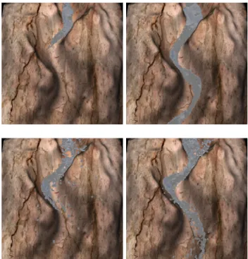
Figure 1 show the result of river in the valley. The fluid flows along to the valley. Since our method can simulate the turbulence, the flow is disturbed. The total number of fluid particles in the scene is about 40,000. The computation time for the simulation was about 15 msec per frame. The calculation of the energy spectrum and the wavelet turbulence requires about 70% of the simulation. We used
marching cubes method to construct the liquid surface mesh and it only took about 15 msec per frame with at most 80k triangles, while we also implemented the marching cubes on GPU.
5 CONCLUSIONS
We have presented a method to simulate turbulent flow using SPH method and a wavelet analysis. Our method directly calculates the turbulent energy by taking a weighted sum of neighborhood parti-cles and adds the turbulence field as a external force. This enables fast simulations that includes various turbulent flow. In addition, we synthesize small vortices, which are dissipated by numerical diffusion, from the energy spectrum using a wavelet turbulent noise based on Kolgomorov’s theory. Moreover, we perform the simula-tion in real-time by using GPU.
There are many directions for future work. We would like to extend the method to handle more small scale turbulent flow by using sub-particles or modifying the surface mesh based on wave equation. For realistic rendering, a bubble, foam and splash are also very important. We will be able to generate these effects based on the turbulence energy.
Figure 1: Water flows in the valley without turbulence (top), and with turbulence (bottom)
REFERENCES
[1] R. L. Cook and T. DeRose. Wavelet noise. In Proc. SIGGRAPH 2005, pages 803–811, 2005.
[2] T. Kim, N. Th¨urey, D. James, and M. Gross. Wavelet turbulence for fluid simulation. In Proc. SIGGRAPH 2008, pages 1–6, 2008. [3] H. Schechter and R. Bridson. Evolving sub-grid turbulence for smoke
animation. In Proc. ACM/Eurographics Symposium on Computer
Ani-mation 2008, 2008.
[4] A. Selle, N. Rasmussen, and R. Fedkiw. A vortex particle method for smoke, water and explosions. In Proc. SIGGRAPH 2005, pages 910– 914, 2005.
[5] J. Stam. Stable fluids. In Proc. SIGGRAPH 1999, pages 121–128, 1999.