Development of Turbidity Monitoring
Methods Over the Coastal Zone Using Aerial
Drone : Case Study in the Estuary of Tokoro,
Hokkaido, Japan, After Low Pressure Events
By
Koji Asakuma*
†, Chihiro Omiya*, Naoto Kida* and Mitsuaki Kitamura**
(Received August 20, 2018/Accepted October 21, 2019)
Summary:The coastal area of Hokkaido bordering the Sea of Okhotsk is famous for cultivating scallops,
however, there have been problems of damage to scallops caused by suspended solids supplied from rivers flowing through these areas after low pressure events ; therefore, the development of a simple and wide-range monitoring method for suspended solids is required. This study aimed to develop a turbidity monitoring method using only an aerial drone, that does not require a special device, targeting the estuary of the Tokoro River flowing through the Tokoro Town located in east Hokkaido. The specifications of commercially available cameras for use by general customers are often not disclosed ; thus, when using such cameras for measurements, it is necessary to analyze their specifications in relation to the object of measurement. The relationship between the turbidity of the turbid water sampled in the estuary of Tokoro River and the reflectance calculated from the images of the river surface photographed with the hovering drone at the site of water sampling were compared using a linear regression model and an exponential regression model. The drone mounted camera detected turbidity with high reliability when using the exponential regression model. As a result of comparing the Root Mean Square Error (RMSE) of both models, the camera mounted on this drone was found to have high reproducibility of high turbidity when using an exponential regression model. However, the precision of this model is slightly insufficient for routine monitoring for daily condition of the river with low turbidity. Thus, improvements such as simultaneous observation of phytoplankton other than inorganic suspended solids are necessary.
Key words:turbidity, suspension solids, aerial drone, Sea of Okhotsk
1. Introduction
The coastal area of Hokkaido bordering the Sea of Okhotsk is famous for its prosperous fisheries. The fisheries catch of the foreshore adjacent to the Sea of Okhotsk reaches 379,000 t per year. The major fishery species captured in this coastal area include scallop (63.6%), salmon (11.4%), and arabesque greenling (9.7%)1).
Because scallops are benthic, growing in fixed coastal areas until harvesting, a locally stable food source is required. Scallops tend to feed on phytoplankton, which are primary producers in the sea, with productivity being driven by the surrounding environment2). Thus, to main-
main-tain the high productivity of phytoplankton in fixed areas, high concentrations of nutrients are required. The coastal area of the Sea of Okhotsk from winter to spring is occupied by the nutrient-rich Okhotsk surface water. However, the nutrient poor Soya warm current flows through these coastal area from early summer to late autumn, from the coast of Hokkaido to nearly 40 km offshore3-6). For example, during summer, nitrates in the
offshore waters (more than 74 km from the coast) exceed 20 µM, whereas nitrates in the Soya warm current are just 2 µM or less7). The area offshore from Tokoro Town,
which is an important fishing area for scallops (Figure 1), has also been filled by the Soya warm water from June
論 文 Article
* **
†
Department of Aquatic Bioscience, Faculty of Bioindustry, Tokyo University of Agriculture Department of Aquatic Bioscience, Graduate school of Bioindustry, Tokyo University of Agriculture Corresponding author(E-mail : [email protected])
onwards7). Therefore, for phytoplankton to grow off-
off-shore from Tokoro after June, a different nutrient source must be supplied to the water mass influenced by the Soya warm current other than the intermediate cold water. For instance, Tokoro River flows through Tokoro Town and supplies an alternative source of nutrients. Tokoro River is the largest river on the coast of east Hokkaido that flows into the Sea of Okhotsk. The catch- catch-ment basin of this river is 1,930 km2, and the average
flow rate is 26.41 m3 s-18). Materials supplied from rivers
include both nutrients and organic and inorganic sus- sus-pended solids, with Tokoro River being no exception. These organic and inorganic suspended solids are preyed on directly by filter feeding bivalves, such as scallops, that inhabit the benthic substrate. Part of the suspended solids is digested and assimilated in the gastrointestinal tract of bivalves, while the remaining organic matter is excreted as feces and the inorganic suspended material is excreted as fake feces. The physical strength of bivalves is weakened by the excretion of fake feces9). It
was confirmed that the ciliary movement of the gill of scallops is noticeably suppressed by suspension containing 0.05% (about 500 degrees in terms of turbidity) mud in sea water10).
Typhoons and explosive cyclones occur under condi- condi-tions of low pressure, and have occurred with greater frequently in recent years11-13). Consequently, there is
concern about scallops being suffocated by increased concentrations of sediments flowing out of rivers in the coastal area of Hokkaido in the Sea of Okhotsk following such events14, 15). However, it is difficult to establish the
extent of damage caused by low pressure weather events in the coastal area of the Sea of Okhotsk. Yet, the munici- munici-palities and fisheries community in this area need to implement methods for estimating damage to the coastal area following such events16). Beside sediments flowing
out from rivers there may also be drifted sediments gen- gen-erated by the rolling up from the seafloor due to waves caused by strong wind, but it is reported that there is almost no impact while the river water is increasing17, 18).
In the case of steady state of the river, there is also the influence of sedimentation of drifted sediments from the seafloor, but this study does not treat it because the study is targeted at the time of river water increases. Observation of plumes of suspended solids from Tokoro River and estuary using satellite images in our previous study showed that the plume spreads about 8 km east- east-wards19). However, because visible to near infrared
wavelengths were used to observe suspended solids, satellite imagery is susceptible to the influence of clouds. In particular, the turbidity of river suspended matter may be instantaneously high during typhoons and explosive
cyclones. Because clouds develop during such events, it is not possible to capture that moment or immediate aftermath of the event with satellite imagery. Sometimes, clouds temporarily clear shortly after typhoons or gales stop blowing, however there is a very low probability of the satellite passing through at that moment. Furthermore, even if the wind subsides, the waves on the coast remain high, making it difficult to observe turbidity from a fishing boat.
In recent years, drones (or Unmanned Aerial Vehicle, UAV) have been effectively used to establish the situation following natural disasters, including volcanic eruptions20, 21),
earthquakes, and landslides22). Drones fly at low altitudes
above the ground, but below the clouds, compensating for satellite observations ; thus, this approach could be used as a substitute for satellite imaging. For oceanic
Fig. 1 Map of Tokoro coastal area on the eastern part
of Hokkaido coast bordering the Sea of Okhotsk.
Fig. 2 Enlarged map of the estuary of Tokoro River,
representing the gray square presented in Figure 1. The drone was launched and landed at the piers in the estuary of Tokoro River, Tokoro Fishing Village Center and Tokoro Fishing Port. The camera icon shows the photographed point using the drone. The dotted line shows a tidal boundary line pre- pre-dicted from the drone image.
and coastal areas, problems remain, including battery duration and susceptibility to weather ; however, high precision observations with drones are possible through the installation of hyperspectral cameras or high resolu- resolu-tion cameras23, 24). For instance, high performance rotary
wing type drones with a resolution of 4 K or more are now available at relatively low costs. These drones are equipped with GPS and autonomous navigation systems, allowing them to fly under certain wind conditions with no problems, and even beginners can easily operate them. It is possible to photograph aerial images showing how plumes spread from the mouth of rivers around coastal areas with drones, even when cloud cover is heavy following the passing of typhoons, as long as the wind is not strong. However, drones developed specifically for sensing are still expensive; low cost drones for beginners are equipped with a CCD camera for general customers. Although CCD cameras for general customers are designed to look vivid with human eyes25), their specifications are
not disclosed, and in many cases the specifications for observation objects are not known. This technique of making the camera image look vivid is implemented with an exponential curve called the γ correction25). Therefore,
to use low cost drones for observations, it is first required to find a calibration method and the value of γ.
This study aimed to estimate the amount of suspended solids flowing from the estuary of Tokoro River following the passing of a typhoon, in addition to estimating the amount of suspended solids that settled in the coastal area offshore of Tokoro Town, using a low cost drone with an installed aerial camera and no special equipment.
2. Materials and Study sites
2. 1 Measurement of the outflow range of suspended solid from the estuary of Tokoro River
To measure the outflow range of suspended solids from Tokoro River, sea surface reflectance was calculated from images photographed with a drone. These aerial images were obtained using a DJI Phantom 4. To convert the photographic images to sea surface reflectance, a standard white board with 99% Lambertian reflectance (Labsphere Inc.) was photographed before the flight, and this white board photographed again after the flight. Figure 2 presents a map of the estuary of Tokoro River. The drone was launched and landed at the piers in the estuary of Tokoro River, Tokoro Fishing Village Center and Tokoro Fishing Port. The lighthouse in the estuary of Tokoro River, the Tokoro Jonan Beach, the lighthouse in Tokoro Fishing Port, the Breakwater of the Lake Inlet of Lagoon Notoro-ko and Cape Notoro were photographed as landmarks. The area of the plume on the surface was measured using the GPS system onboard the drone
combined with positional information of landmarks on the map. The tidal boundary information was separated from the sea surface color of the drone RGB images (e.g., blue color of the ocean sea surface or brown color of turbid water from the river).
Aerial imagery using the drone was collected on October 24, 2017, immediately after Typhoon Lan (Typhoon No. 21), and October 27, three days after the typhoon, when conditions had calmed down. On October 31, 2017, only water surface imagery of the river was obtained with hovering of the drone because the wind speed exceeded 7 m s-1 due to the low pressure devel-
devel-oped in the Sea of Okhotsk. To document the steady state of the estuary, water surface imagery was obtained on September 28, 2017, December 4, 2017, April 13, 2018 and April 20, 2018 by hovering the drone. Thus, aerial imagery was obtained with the hovering of the drone, from which the turbidity and water surface reflectance of the estuary were measured.
2. 2 Measurement of turbidity, sedimentation rate and particle size of suspended solids
To determine the amount of actual suspended solids flowing out from Tokoro River, the surface water of the estuary of the river was sampled with a hydrochloric acid washed bucket, in accordance with the drone flight. The sampled water was analyzed with a transmitted beam type digital color turbidimeter, WA-PT-4DG (Kyoritu Chemical Check Lab., Corp.), calibrated with polystyrene particles. The dry weight concentration was measured for water sampled on October 31, 2017, December 4, 2017, April 13, 2018 and April 20, 2018. A total of 500 mL turbid water was passed through the Whatman GF/F filter, then the dry weight was weighted from the difference in weight of the filter before and after filtration.
The sedimentation rate was measured using river water sampled on October 31, 2019. The sampled water was dispensed in a 500 mL graduated cylinder (45 cm height). Then, 10 mL water on the surface was sampled with an auto pipette. The turbidity of surface water was measured with a digital color turbidity meter. Turbidity was measured at set time intervals until 2 degrees turbidity was reached26). This value (2 degree turbidity)
is the costal revetment standard in Japan that is assumed not to affect coastal fisheries. According to the environ- environ-mental standards of rivers in Japan, the turbidity of less than 25 degrees is not considered to impact river water quality27).
The particle size of the suspended solids was measured using river water sampled on the same day to measure the sedimentation rate. The sampled water was poured
in a 500 mL graduated cylinder that was prepared sepa- sepa-rately to that used to measure the sedimentation rate. After allowing the sample to stand for 20 days, supernatant water was gently discharged with a tube and concentrated to 25 mL. Then, 0.5 mL of this concentrated water sample was pipetted out with a micro pipette and the number of particles for each particle size was counted with a bio- bio-logical microscope (Olympus CX41 Upright Microscope). A 0.5 mL volume of the concentrated water sample was fractionated by 1,000 fractions. The size of each fraction was 5 µm square. The number of particles in each fraction was 524. One-hundred particles were randomly selected, and particle size was measured.
3. Results
3. 1 Influence range of turbid water from the mouth of Tokoro River
Figure 3 shows a situational view photographed with the drone of the estuary of the Tokoro River on October 24, after Typhoon Lan passed through. The tidal boundary between the density of the turbid river water and the density of the clear seawater was visually confirmed by flying the drone on the west side and north side of the lighthouse (Point E in Figure 2 ; Figure 3), and was located near Tokoro Public Pool on Jonan Beach 500 m west of the lighthouse (Point J in Figure 2 ; Figure 4) and 1750 m north of the fishing village center (Point V in Figure 2). By turning the drone towards the tidal boundary line, this boundary line seemed to draw a clean arc without interruption. Likewise, the tidal boundary line was delin- delin-eated 2,500 m on the east side of Tokoro Fishing Port, before the inlet of Lagoon Notoro-ko (Point P in Figure 2 ; Figure 5). Thus, suspended solids existed on the sea surface for about 5 km in a west to east direction from 500 m west of the estuary (Point J in Figure 2) to 2500 m east of the Fishing Port (Point P in Figure 2), and 1750 m in a south to north direction from the Fishing Village Center to 1750 m north of this center (Point V in Figure 2). The Nadia image over each tidal boundary line on October 24 is shown in Figure 6, and a similar image on October 27 is shown in Figure 7. Compared to Figure 6, the contrast between the inside and the outside of the boundary line clearly decreased.
3. 2 Calculating turbidity from drone imagery
Figure 8 is the aerial picture of the work scenery of surface water sampling photographed with the drone on October 24, 2017. The square area over the river surface and the standard white board image were cropped to 100×100 pixels from Figure 8 to obtain each pixel value. Nine of the pixel values of the Tokoro river estuary image were divided by the pixel values of the white
board, and were then multiplied by 255 to obtain 8-bit normalized imagery (Hereinafter, all the pixel values indicate normalized values). Histograms were created from the R, G, and B channel images cut into squares from Figure 8 ; These histograms are shown in Figure 9. The average pixel value of each R, G, and B channel in Figure 8 was 132.4±3.9, 116.5±3.9, and 89.7±3.8, respec- respec-tively. In comparison, turbidity based on the turbidimeter
Fig. 3 Situational view of the estuary of Tokoro River
photographed with the DJI Phantom 4 on October 24, 2017.
Fig. 4 Image of the tidal boundary between turbid water
and seawater fronting Tokoro Town Public Pool at Tokoro Jonan Beach on the west side of the estuary of Tokoro River on October 24, 2017.
Fig. 5 Image of the boundary between turbid water and
seawater at the Inlet of Lagoon Notoro-ko Tokoro on the east side of Tokoro Fishing Port on October 24, 2017.
of the water sampled on the estuary surface on this day was 60.0 degrees. All average normalized pixel values for R, G, and B are presented as xR, xG, and xB, respectively.
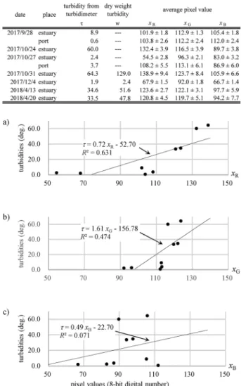
The turbidity observed with the turbidimeter is repre- repre-sented by τ, while the turbidity based on the ratio of the dry weight of the suspension in 1 L water is represented by w. Table 1 presents the xR, xG, and xB obtained from
Table 1 Average normalized pixel values of xR, xG, and xB
for each R, G, and B channel obtained from the drone, turbidity τ, and dry weight turbidity w.
Fig. 10 Relationship between xR, xG, xB and τ presented
in Table 1. Solid line shows the regression line between the pixel values and τ. a) R channel, b) G channel and c) B channel.
Fig. 6 Image showing the nadir view near the tidal
boundary line between turbid water and clear seawater on October 24, 2017. a) Above the estuary. b) Offshore from Tokoro Jonan Beach. c) Offshore from Tokoro Fishing Village Center. d) East side of Tokoro Fishing Port, near the Lagoon Notoro-ko inlet. Squares in the figure were used as test site to calculate turbidity.
Fig. 7 Drone image of the nadir on October 27, 2017,
obtained at the same place as in Figure 6.
Fig. 8 Drone image when sampling surface water on
October 24, 2017.
Fig. 9 RGB Composed image and each image of the R,
G, and B channels and each histogram based on the white square shown in Figure 8.
the drone images using the same method on October 24, and τ and w obtained by water sampling during the observation period. The highest τ during this period was 64.3 degrees in the estuary, which was recorded on October 31, just after the low pressure from the Sea of Okhotsk. The xR, xG, and xB were 138.9±9.4, 123.7±8.4,
and 105.9±6.6, respectively, on this date. The lowest τ was 0.6 degrees in the port on September 28. The xR, xG,
and xB were 103.8±2.6, 112.2±2.4, and 112.0±2.4, respec-
respec-tively, on this date. Regression lines were calculated from relationships between each xR, xG, and xB and τ from
Table 1. These regression lines are shown in Figure 10. The regression formula of xR and τ was expressed as :
τ=0.72 xR-52.70 (R2=0.631, P<0.01)…(1).
The root means square error (RMSE)28) is often used to
indicate precision in remote sensing (rather than the standard deviation), and was RMSE=14.69 when applying formula (1). The regression formula of xG was expressed
as :
τ=1.61 xG-156.78 (R2=0.474, P<0.05)…(2).
The RMSE in formula (2) was RMSE=17.54. The regres- regres-sion formula of xB was :
τ=0.49 xB-22.70 (R2=0.071, P=0.49>0.05)…(3).
Thus, xB showed little correlation with τ. Based on these
results, xB was excluded from the subsequent discussion.
The estimated value of τ was expressed as a function of the linear combination of xR and xG :
τ=aR xR+aG xG+b. …(4)
The optimal parameter found by the least squares method using MS-Excel’s solver by placing τ, xR and xG in Table 1
to formula (1) was aR=0.987, aG=-0.674 and b=0.060.
However, since aG became negative, the multiple regres-
regres-sion analysis of τ and xR, xG was performed. The P value
for xR in this analysis was 0.01, but the P value for xG was
0.3>0.05. This result indicates the confidence interval of xG contains 0.
Next, to suppress the vivid correction for the camera, the method of estimation was modified from the linear combination regression to exponential curve regression. Since this suppression correction is expressed by the in- in-verse operation of gamma correction, so the corrected xR′
is expressed with the pixel value xR and the parameter
of gamma correction for R channel γR :
Using this corrected pixel value in R channel with the regression parameters cR and dR, rewriting the regression
equation for τ can be expressed as :
…(5)
Figure 11 shows the relationship for the γ corrected pixel values of xR and xG with τ. In the curve shown in Figure 11,
the determination coefficient R2=0.936 was maximized
when γR=0.147, cR=17.65 and dR=0.0. The P value was
P<0.01 and RMSE=2.04 at this case. Similarly, by re- re-placing cR, xR, γR and dR with cG, xG, γG and dG respectively
in the curve shown in Figure 11 b), the determination coefficient R2=0.936 was maximized when γ
G=0.066, cG=
1.27×10⁴, d
G=0.0, P<0.01 and RMSE=4.81.
3. 3 Relationship between turbidity τ measurements based on the turbidimeter and the dry weight turbidity w of suspended solids
The turbidity τ obtained with the turbidimeter was an optically relative value determined from the polystyrene standard. To quantitatively evaluate the inflow of various suspended substances contained in river water, it must be converted to the weight of the actually flowing sus- sus-pended solids. Figure 12 shows the relationship between
τ obtained with the turbidimeter and the dry weight
turbidity w of the suspended solids in sampled water (shown in Table 1). The solid dotted line in this Figure shows the linear regression formula :
w=2.02 τ-10.09 (R2=0.961, P=0.02<0.05)…(6).
The τ estimated from the drone using formula (5) was converted to w of suspended solids using this formula (6).
3.4 Estimation of sedimentation rate of suspension
The number of particles of the sampled water in the estuary of the Tokoro river counted with the microscope is shown in Table 2. Assuming that the number of particles N(D) follows a bi-modal normal distribution of particle diameter D in the sampled water, this particle distribution could be expressed as :
Fig. 11 Relationship of the γ corrected xR and xG with τ.
…(7) where μ1 is the mode diameter of small particles, σ1, is
the standard deviation of small particles, μ2 is the mode
diameter of large particles, and σ2 is the standard devia-
devia-tion of large particles. When formula (7) was matched to the counted number of particles shown in Figure 13 by the least squares method, this size distribution has two peaks, the optimal parameters of μ1=5.0, σ1=1.3, μ2=15.0,
and σ2=5.1 were calculated. The bi-modal particle size
distribution curve of these parameters is shown by a dotted line in Figure 13.
Figure 14 shows the change in the time dependent turbidity of surface water sampled in the estuary of Tokoro River on October 31, 2017, based on the method presented in section 2.2. From the observation results of particle distribution, a sedimentation velocity of two particles expressing a decrease in τ with time t was described as :
…(8)
where α1 and β1 are the decreasing parameters of large
particles and α2 and β2 are the decreasing parameters of
small particles. The optimum value of formula (8) using the least squares method in relation to measured turbidity was shown as α1=16.40, β1=-6.90×10⁻³, α2=24.09 and
β2=-1.16×10⁻¹ in Figure 14. The τ calculated using
formula (8) did not decline to 0.0, requiring 750 h (31 days) to reach <0.1. If α2=0 was substituted, the τ of
large particles only could be calculated, which required 70 h to reach <0.1. Substituting the mode diameter 5.0 µm of small particles obtained the above results in the Stokes equation29), where the average particle density
was 1.11 g cm-3. The terminal sedimentation velocity of
small particles was 1.67×10⁻⁵ cm s-1 or 1.44×10⁻² m day-1.
Similarly, the particle density of large particles was 1.13 g cm-3 with the mode diameter of 15.0 µm. The terminal
sedimentation velocity of large particles was 1.77×10⁻⁴
cm s-1 or 1.53×10⁻¹ m day-1.
4. Discussion
In order to estimate turbidity τ from aerial drone images, the linear regression model and the exponential regression model, which were calculated from each pixel value of xR,
xG, and xB photographed with the drone, were provided
and compared. In the case of the linear regression model, significant correlation was found between each xR and xG
with respect to τ from the results of formula (1) and (2) in Section 3.2, but xB in formula (3) was not significant for τ.
Thus, xB could not be used to estimate τ in the linear
Fig. 12 Relationship between the turbidity τ and
the dry weight turbidity w in the estuary of Tokoro River.
Table 2 Number of particles of suspended solids in
the estuary of Tokoro River on October 31, 2017. D µm is particle diameter and, Na is
the number present in 100 particles and Nv
is the number of particles in 1.0 L.
Fig. 13 Bi-modal particle size distribution of the sus- sus-pended solids in the surface waters at the estuary of Tokoro River on October 31, 2017.
Fig. 14 Variation in the turbidity of the surface water
of the estuary of Tokoro River over time on October 31, 2017. Solid line shows the approximate curve of the relationship between lapsed time and turbidity.
regression model. The coefficient of determination be- be-tween xR and τ was 0.631, the coefficient of determination
between xB and τ was 0.474 ; That means the correlation
between xR and τ was larger than the correlation be-
be-tween xG and τ. In addition, when xR and xG were linear
combined shown in formula (4), there was a problem that the coefficient of the G channel became a negative value. The result shows that τ is difficult to express as the simple linear combination model of xR and xG. Therefore, when τ
is expressed by the linear regression model, it is desirable to express only by xR shown in formula (1). From Figure
10 B), it is obvious that xB is not significant for τ even in
exponential regression. In the case of the exponential regression model, significant correlation was found between each xR and xG with respect to τ from the results of for-
for-mula (5). The RMSE when using xR was 2.04 and the
RMSE when using xG was 4.81, so there was a 2.4 times
difference in precision. For this reason, the two models consisted of only xR. The RMSE of the linear regression
model was 14.69 and the RMSE of the exponential curve model was 2.04, so the exponential curve model became valid. Since the expanded uncertainty of this model was 2 RMSE=4.08, it is possible to estimate the environmental standard of rivers of 25 degrees for highly concentrated rivers. However, in order to detect turbidity of 2 degrees that is not affected by the fishery, the expanded uncer- uncer-tainty should be below 1.0, so the precision of this model is not enough. In order to estimate the low turbidity range, there should be an accumulation of observation data and increased precision in the future. On the other hand, the reason why aG the coefficient of xG became negative in
spite of the xG and τ small correlation could be that the
multiple regression parameter aG may have been adjusted
to minimize RMSE. In general, inorganic suspended solids such as soils reflect red light more strongly than green light30), but Chlorophyll a in phytoplankton has the
opposite spectral characteristics due to photosynthesis2).
Thus, in order to increase the precision of estimating τ, it is necessary to collect chlorophyll a concentration data. Finally, the example of applying the w estimation model provided in formula (5) and (6) to drone observation over and around the estuary of the Tokoro river was examined. Table 3 shows pixel values in the white square area in Figs 6 and 7 and the estimated w calculated with formula (5) and (6) from the pixel value xR. Figure 15 a) shows
the distribution of w calculated by interpolation and extrapolation with GMT31), a geographic information sys-
sys-tem, from the drone imagery on October 24, 2017. The difference in w between the inside and outside of the tidal boundary line was large at all three locations of Jonan Beach, the fishing village center and the east coast of the fishing port. The w inside the boundary line indi-
indi-cated higher than the river environmental standard of 25 degrees at all three locations of Jonan Beach, the fishing village center and the east of the Tokoro fishing port. On the other hand, w inside the tidal boundary line indicated lower than 2 degrees of the coastal revetment standards at all three locations. In this result, on October 24, there were large differences in w between the high turbidity water area and other areas. The high turbidity area exceeding 25 degrees covered 28.5% of the sea area 7.2 km×4.5 km (32.0 km2) from the river estuary. The w=
55.1 degrees in the northern tidal boundary of the high turbidity area and w=45.1 degrees in the eastern tidal boundary were slightly lower than w=64.8 degrees in the vicinity of the estuary. However, w=111.1 degrees in the western boundary was higher than the turbidity in the vicinity of the estuary. Figure 15 b) shows the distribution of the surface turbidity on October 27 calculated from the drone image similar to a). Compared to October 24, the w inside the tidal boundary line was lower than 25 degrees in all three places. The difference of the w between the outside and the inside of the tidal boundary line became small in all places. However, the value of the w=16.5 degrees in the offshore of Jonan Beach and w=22.4 degrees in the eastern offshore of Tokoro fishing port indicated higher values than the value of the w=5.5 degrees in the vicinity of the estuary. From these observation examples, there were 2.8 times a clear difference between the average surface turbidity 50.3 degrees in the high turbidity area
Table 3 stimated w calculated with the formula (5) and
(6) from the xR from sample areas from Figures
6 and 7. the value of w remains including the uncertainty RMSE (=2.04). The asterisk * rep- rep-resents when w was less than 2 RMSE. The double asterisk ** represents when w was less than RMSE. Black fills indicate w>25 and light gray fills indicate w>2.
on October 24 after passing the low pressure and the surface turbidity 17.7 degrees after 3 days.
Since the time for large particles to settle from the surface layer is 70 hours from the result from section 3.4, the large particles supplied from the Tokoro River in these three days are considered to have settled immedi- immedi-ately from the surface layer. The sedimentation flux of large particles was 18.57 g m-2 day-1 on October 24, 2017
and 19.74 g m-2 day-1 October 31. Each flux was calculated
by multiplying w in Table 1 by the terminal sedimentation velocity. The w on October 24 was converted from tur- tur-bidity and formula (6). The sedimentation flux in these cases are almost twice as fast as the previously known the normal state sedimentation flux of 9.24 g m-2 day-1
offshore of Lagoon Notoro-ko32). However, the difference
between the inside and outside of the tidal boundary line was small on October 27. It is reported that the suspended solids derived from rivers are mixed with seawater slowly after diffusing to the surface once33). The small particles
could stay on the surface for more than 31 days, from the result of section 3.4, so the small particles remaining on the sea surface are considered to have mixed with sea- sea-water and diffused across the tidal boundary line. This drone observation seems to have captured the diffusion of the suspended solids before and after being mixed with seawater in the surface layer.
The estuary of the Tokoro River faces the northeast as shown in Figure 2 and the Soya Warm Current flows toward the east on the north side of the estuary. Under this condition, suspended solids should flow northeast. However, the results shown in Table 3 indicated that the turbidity on the west side was higher than the turbidity of the vicinity of the estuary, the source of suspended solids. There is a shore reef on the shallow sea floor just east of the estuary, and the flow of the river is blocked by this shore reef, once heading west, then heading to north34). For this reason, it is considered that suspended
solids flowing from the estuary stayed in the vicinity of the western tidal boundary line. The cause of the higher turbidity in the vicinity of the west boundary line than the turbidity of the estuary cannot be identified, but there may be factors other than the influence of suspended solids from the estuary because of the nearness to the inlet of the Lagoon Notoro-ko.
It is difficult to observe such as these two above instantaneous phenomena with satellites and ship obser- obser-vation. In order to take advantage of the convenience of drone observation for environmental monitoring of the coastal area around this estuary in the future, real-time calculation of the turbidity estimation model and continuous shooting with movies will be necessary.
Acknowledgement
The authors would like to thank Dr. K. Sakaguchi of the Aquaculture Fishery Cooperative of Saroma Lake for providing advice on the site where the drone was operated.
References
1) Hokkaido Government, Profile of Hokkaido Fisheries, <http:// www.pref.hokkaido.lg.jp/sr/sum/grp/02/AP_05_2010_ Fisheries_in_Hokkaido.pdf> (Last Access May 29, 2018) 2) Lalli C and Parsons T (1997) Biological Oceanography :
An Introduction, Second Edition. Elsevier Butterworth Heinemann, Oxford, pp. 40-73.
3) Aota M (1971) Study of the Variation of Oceanographic Condition to the North East off Hokkaido in the Sea of Okhotsk III. Low Temp. Sci. Ser. A Phys. Sci. 29 : 210-224.
4) Takizawa T (1982) Characteristics of the Soya Warm Cur- Cur-rent in the Okhotsk Sea. J. Ocea. Soc. J. 38 : 281-292. 5) Aota M, Ishikawa M and Uematsu E (1988) Variation in
Ice Concentration off Hokkaido Island. Low Temp. Sci. Ser. A Phys. Sci. 47 : 161-175.
6) Maita Y and Toya K (1986) Characteristics on the Distri- Distri-bution and Composition of Nutrients in Subarctic Regions. Bull. J. Soc. Fish. Ocea. 50 (2) : 105-113.
7) Kudo I, Frolan A, Takata H and Kobayashi N (2011) Ocean-
Ocean-Fig. 15 Surface distribution of w calculated using the
GMT from the drone imagery. a) On October 24, 2017. b) On October 31, 2017.
ographic Structure and Biological Productivity in the Coastal Area of Okhotsk Sea. Bull. Coast. Ocea. 49 (1) : 13-21.
8) Hokkaido Regional Development Bureau, Ministry of Land, Infrastructure, Transport and Tourism Japan <https:// www.hkd.mlit.go.jp/ab/tisui/v6dkjr00000006jx.html> 9) Wotton R S, Malmqvist B (2001) Feces in Aquatic Ecosys-
Ecosys-tems : Feeding Animals Transform Organic Matter into Fecal Pellets, which Sink or are Transported Horizontally by Currents ; these Fluxes relocate Organic Matter in Aquatic Ecosystems. BioScience 51 (7) : 537-544.
10) Yamamoto G (1956) On Behavior of the Scallop under some Environmental Conditions, with Special Reference to Effects of Suspended Silt, Lack of Soluble Oxygen and others on Ciliary Movement of Gill Pieces. J. J. Ecol. 5 (4) : 172-175.
11) Japan Meteorological Agency, Latest Weather, <https:// www.data.jma.go.jp/fcd/yoho/typhoon/statistics/landing/ landing.html>
12) Kitano Y and Yamada T (2016) The Relationship between Explosive Cyclone through Northern Japan and Pacific Blocking. J. J. Soc. Civil Eng. Ser. B1 72 (4) : 121-126. 13) Kyusyu Univ., Explosive Cyclone Database, <http://fujin.
geo.kyushu-.ac.jp/meteorol_bomb/index.php>
14) Weekly Paper Suisan Shinbun, <http://suisan.jp/article- 7483.html> (Last access November 20, 2017).
15) Ministry of Agriculture, Forestry and Fisheries, <http:// www.maff.go.jp/j/saigai/typhoon/20171106.html> (Last access November 20, 2017)
16) Fishing Communities Promotion and Disaster Prevention Division, Fisheries Infrastructure Department, Fisheries Agency Japan, <http://www.jfa.maff.go.jp/j/bousai/ hamaplan/hokkaido_koikihamaplan.html> (Last access November 20, 2017)
17) Fukushima H, Kashiwamura M, Yakuwa I and Takahashi S (1964) A Study of the mouth of the Ishikari river. Proc. Coast. Eng. Comm. J. Soc. Civil Eng. 11 : 137-146. 18) Funaki J and Shinme R (1999) Sediment diffusion from
Mukawa River to ocean after the 1997 Flood. Proc. Conf. Hydr. Eng. J. Soc. Civil Eng. 43 : 449-454.
19) Asakuma K, Kenjyou Y and Shima T (2016) Study of the classification method for the costal water in an outfall area along the Hokkaido coast in the Okhotsk Sea from satellite imagery. Low Temp. Sci. 74 : 85-93.
20) Ohminato T, Kaneko T, Koyama T, Watanabe A, Yasuda A, Takeo M, Honda Y and Iguchi M (2011) Volcano Obser- Obser-vations Using an Unmanned Autonomous Helicopter : seismic observations near the active summit vents of Sakurajima volcano, Japan. Geophys. Res. Abst. 13 : EGU2011-2855.
21) Koyama T, Kaneko T, Ohminato T, Yanagisawa T, Watanabe A and Takeo M (2013) An aeromagnetic survey of Shinmoedake volcano, Kirishima, Japan, after the 2011 eruption using an unmanned autonomous helicopter. Earth Planets Space 65 : 657-666.
22) Niethammer U, James M R, Rothmund S, Travelletti J and Joswiga M (2012) UAV based remote sensing of the Super-Sauze landslide: Evaluation and results. Eng. Geology 28 (9) : 2-11.
23) Lomax A S, Corso W and Etro J F (2005) Employing Un- Un-manned Aerial Vehicles (UAVs) as an element of the Integrated Ocean Observing System. Proc. OCEANS 2005 MTS/IEEE 1 : 184-190.
24) Klemas V V (2015) Coastal and Environmental Remote Sensing from Unmanned Aerial Vehicles : An Overview. J. Coastal Res. 31 (5) : 1260-1267.
25) Praveen C, Marcelo B, David K and Corral J V (2015) A Tone mapping operator based on Neural and Psychophysical Models of Visual Perception. Proc. SPIE 9394, Human Vision and Electronic Imaging XX : 93941I.
26) Overseas Environmental Cooperation Center, Japan, <https:// www.env.go.jp/earth/coop/coop/document/04-wpctmj1/04-wpctmj1.pdf> (Last Access December 11, 2017)
27) Ministry of the Environment Government of Japan, Envi- Envi-ronmental Standard about Preservation of Living Envi- Standard about Preservation of Living Envi- Envi-ronment <https://www.env.go.jp/kijun/pdf/wt2-1-1.pdf> 28) Yong H K, Jungho I, Ho K H, Jong-Kuk C and Sunghyun H
(2014) Machine learning approaches to coastal water quality monitoring using GOCI satellite data. GIScience & Remote Sens. 51 (2) : 158-174.
29) Mouri M and Fujii S (1997) Analysis on settling velocity distribution of suspended matter determined by the Plural Settling Cylinders Method. J. J. Soc. Water Env. 20 (12) : 838-844.
30) California Institute of Technology, The ECOSTRESS spectral library, <https://speclib.jpl.nasa.gov/>
31) GMT-The Generic Mapping Tools, <http://gmt.soest.hawaii. edu/> (Last Access April 21, 2018)
32) Miyazono A, Tada M and Komatsu T (1995) Growth of Scallops (Patinopecten yessoensis) in sowing culture grounds around the Abashiri Bay in relation to water and sediment flux. Bull. J. Soc. Fish. Ocea. 59 (4) : 389-397.
33) Ishii J, Okada S and Iwata K (1977) The Suspended Matter in Sea Water in the Bay of Ishikari, Hokkaido, North Japan. Earth Sci. 31 (1) : 19-33.
34) Yamashita T, Oshida R, Tomisawa S, Sato M, Tokisawa T and Yamagami Y (2014) Influence of the Climate Change on Sediment Transport around the Second Inlet of Saroma Lake. J. J. Soc. Civil Eng. Ser. B2 70 (2) : 606-610.