Contact, network, people, and geographical space : Perspectives on the S&K network method and the Linguistic Atlas of Japan Database

全文

(1)Dialectologia. Special issue, 8 (2019), 117-144. ISSN: 2013-2247. Received 23 October 2019. Accepted 7 November 2019.. CONTACT, NETWORK, PEOPLE, AND GEOGRAPHICAL SPACE: PERSPECTIVES ON THE S&K NETWORK METHOD AND THE LINGUISTIC ATLAS OF JAPAN DATABASE Yasuo KUMAGAI National Institute for Japanese Language and Linguistics ** [email protected]. Abstract This paper discusses two research projects related to Takesi Sibata and Willem A. Grootaers: The S&K network method and the Linguistic Atlas of Japan Database (LAJDB). The S&K network method was proposed by Sibata to objectively divide dialect areas. The original idea demonstrated by Sibata involved dialect division through a network of linguistic similarities drawn on a map. The LAJDB is a project that aims to digitally render the entirety of the information contained in the Linguistic Atlas of Japan (LAJ). The LAJ is Japan’s first nationwide linguistic atlas created on the basis of a linguistic geographical survey. Sibata and Grootaers were pivotal to the project. This paper focuses on several concepts and perspectives that were utilized for these projects: contact, network, people, and geographical space. These aspects were essential to the advancement of these research initiatives and are closely linked to their common spirit of linguistic studies. Keywords contact, network, geographical space, population distribution, dialect area. *. * National Institute for Japanese Language and Linguistics, 10-2 Midori-cho, Tachikawa City, Tokyo, 190-8561 Japan.. 117 ©Universitat de Barcelona.

(2) Yasuo KUMAGAI. CONTACTO, RED, PERSONAS Y ESPACIO GEOGRÁFICO: PERSPECTIVAS SOBRE EL MÉTODO DE RED S&K Y LA BASE DE DATOS DEL ATLAS LINGÜÍSTICO DE JAPÓN Resumen Este artículo discute dos proyectos de investigación relacionados con Takesi Sibata y Willem A. Grootaers: el método de red S&K y la base de datos del Atlas Lingüístico de Japón (LAJDB). Sibata propuso el método de red S&K para dividir objetivamente las áreas dialectales. La idea original demostrada por Sibata involucraba la división del dialecto a través de una red de similitudes lingüísticas dibujadas en un mapa. El LAJDB es un proyecto que tiene como objetivo reproducir digitalmente la totalidad de la información contenida en el Atlas Lingüístico de Japón (LAJ). El LAJ es el primer atlas lingüístico nacional de Japón creado sobre la base de una encuesta geográfica lingüística. Sibata y Grootaers fueron fundamentales para el proyecto. Este documento se centra en varios conceptos y perspectivas que se utilizaron en dichos proyectos: contacto, red, personas y espacio geográfico. Estos aspectos fueron esenciales para el avance de estas iniciativas de investigación y están estrechamente vinculados a su espíritu común de estudios lingüísticos. Palabras clave contacto, red, espacio geográfico, distribución de la población, área dialectal. 1. Introduction Takesi Sibata (1918-2007) was a pioneer of sociolinguistics and linguistic geography in Japan (Sibata 1969, 1978, etc.). Willem A. Grootaers (1911–1999) was a Belgian priest and dialectologist who contributed significantly to the development of Japanese linguistic geography (Grootaers 1976, etc.). This paper is to be incorporated in a special issue dedicated to Willem A. Grootaers and Takesi Sibata, and in it, I employ my own research experiences to discuss two research projects related to the two scholars: (1) the S&K network method and (2) the Linguistic Atlas of Japan Database (LAJDB). In my discussion, I focus on several concepts and the perspectives such as contact, network, people and geographical space that were utilized in the projects. These frameworks were essential to the advancement of these research initiatives and are closely linked to their common spirit of linguistic studies.. 118 ©Universitat de Barcelona.

(3) Dialectologia. Special issue, 8 (2019), 117-144. ISSN: 2013-2247. Sibata explained his vision of linguistic geography in the final chapter of Method of Linguistic Geography (Sibata 1969: 182-195). The last page offers perspectives such as “dialect and people”, “geographical distribution as the base of the method of linguistic geography”, “language, culture, history, and society”, “human psychology of using language and creating language”, “human relations in society”, and so on (Sibata 1969: 195). In the section entitled “the fundamental hypothesis of linguistic geography,” he elucidated the nature and the origin of linguistic geography’s dialect diffusion from the perspective of contact and communication between persons (Sibata 1969: 16-17). These perspectives indicate the concepts necessary for the investigation of dialect distribution: contact, network, people, and geographical space. These notions are essential to the advancement of both the S&K network method and the LAJDB.. 2. Contact, network, and geographical space 2.1 Network of linguistic similarities drawn on a map The S&K network method (Sibata & Kumagai 1984, 1993, etc.) was originally proposed by Sibata to provide a new method for the objective division of dialect areas. The S&K network method was developed through a collaborative research project conducted by Sibata and Kumagai, the author of the present paper. We began developing our ideas in the 1980s (Sibata 1982b, etc.)1 and the research endeavor has continued since then (Kumagai 2016, etc.) Sibata’s original idea was to draw a dialect division through a network of linguistic similarities drawn on a map. Figure 1 (Sibata 1982b: 21) shows the first map drawn in the process of the development of the method. This map was grounded in a linguistic geographical survey conducted by Sibata and others in 1977, 1978 and 1979 1. Sibata (1982a, b), Sibata (1984: 322-426, 1988b: 514-523, 536-537, 557-563), Kumagai & Sibata (1987), Sibata & Kumagai (1984, 1985, 1987, 1993, etc.); Sibata & Kumagai (1993) provides an overview of our development until then.. 119 ©Universitat de Barcelona.

(4) Yasuo KUMAGAI. in Amami-Ôshima, an island located in the south-western segment of Japan (Sibata 1984). Every single human settlement (143 localities) was surveyed. Henceforth, we will refer to this Linguistic Atlas of Amami-Ôshima survey as the LAA.2 Figure 2 illustrates a map from the LAA. We prepared two types of data set: phonological items and lexical items. The data set used in this figure comprises 177 phonological items (LAA data). The degree of linguistic similarities between two localities was measured by the number of the word forms (linguistic features) shared by them. This measure was termed Number of Common linguistic features (NC). A straight line was used to connect any pair of localities on the map whose NC were not less than 21. Figure 1 displays a concentration of the similarity network of an area corresponding to the south-west of Amami-Ôshima named Nishimagiri, an ancient administrative district of the Ryûkyû and Simazu eras that extended from the end of the 15th century to mid18th century (Sibata 1982b: 20-21, 1984: 32-34). The first results conformed to Sibata’s expectations. Later, the network representation shown in Figure 1 was named NT-1.. Figure 1. Network of linguistic similarity drawn on a map (Sibata 1982b:21).3. 2. Figure 2. A map from Linguistic Atlas of Amami-Ôshima (Sibata 1984: 238).. The outcomes of the early stage of our development was included in Sibata (1984: 322-426). This first network map was drawn by hand and there is one link error in this figure. There is a link between 5762 and 5778 but the correct link is between 5762 and 5783. The Figure 1 is original one (Sibata 1982b). In Sibata & Kumagai (1984, 1985), network maps were drawn by computer and the error of Figure 1 was corrected.. 3. 120 ©Universitat de Barcelona.

(5) Dialectologia. Special issue, 8 (2019), 117-144. ISSN: 2013-2247. Dialect division has been a major concern for Japanese dialectology since the beginning of the discipline (Kato 1977: 41-82, Inoue 2001: 3-25). The first generation of the methods of dialect division involved drawing dividing lines based on a comprehensive and integrated judgment that was more subjective than analytical. The second generation was represented by the isogloss method. Although this technique is objective and analytical, drawing the isogloss represents difficulties and ambiguities. Sibata proposed the S&K network method as a third generation approach to an objective dialect division which would resolve the difficulties of the isogloss method (Sibata 1988b: 514-515). At the same time, he raised a problem relating both to the isogloss technique and the S&K network method: It is a fundamental standpoint of linguistic geography to focus on the people who inhabit the land and the words they speak. Linguistic geography sheds light on the diversity of the words by place and people. Then, it raises a general linguistic problem such as how to find the commonality in the diversities and how to relate the diversities and the commonalities. Synthesis of dialect distribution maps is an answer but we should find yet another answer someday (Sibata 1988b: 563-564).4. Soon after the beginning, a second aim was added to the development efforts: the advancement of a method that would enable the observation of varying degrees of linguistic similarities among localities and that would afford the scrutiny of how these localities formed clusters on a map.5 As the methodology has evolved, the latter aim has gained the greater focus. We introduced a threshold condition, Lcond (Level conditioned), to the S&K network method to observe the varying degree of similarities. We named this revised NT-1 NT-1(r)n, where “n” indicates the measure used, NC. Besides the abovementioned NC, we defined DC (distance of NC) to measure linguistic similarities 4. The text first appeared in 1984 in Koza Hogengaku vol.2, Tokyo:Kokushokankokai. The first map of similarity network was drawn by hand. It was exploratory. Only the calculation of the similarity matrix of the LAA was done by computer. For the second aim, full utilization of computer is indispensable. It was before the rapid development of computer. At first, we used main frame computer of a computer center, then workstation and, finally, personal computer. The figures in this paper include the outputs of these different periods.. 5. 121 ©Universitat de Barcelona.

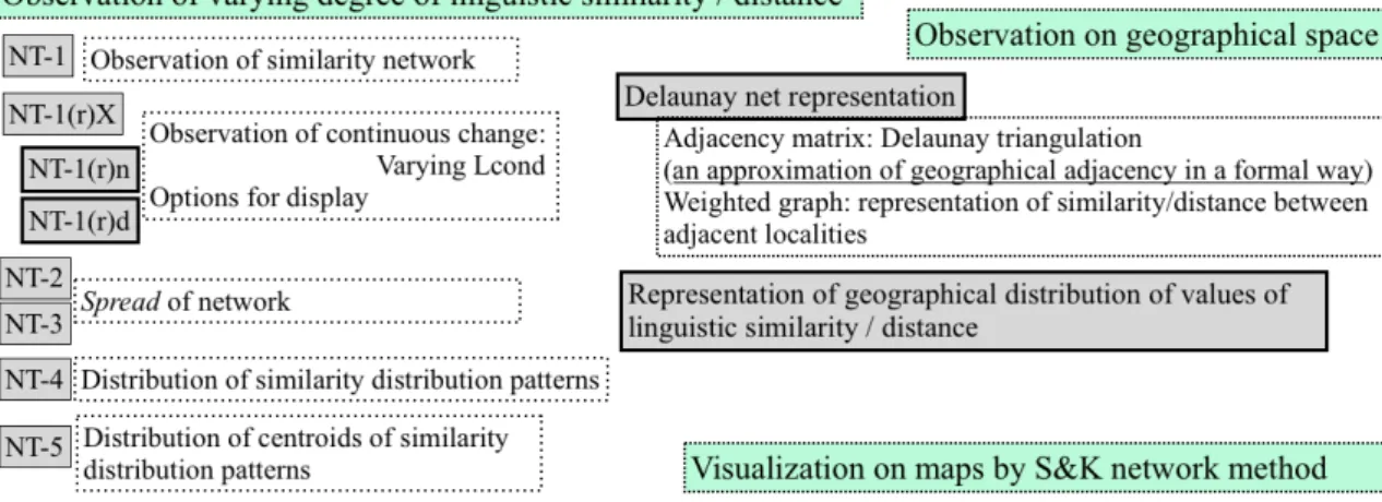
(6) Yasuo KUMAGAI. (Kumagai & Sibata 1987, Sibata & Kumagai 1987). The distance DC between any two localities was measured by the Euclidean distance between the two NC distribution patterns. DC was defined as follows:. where n represented the number of localities. The values of DC were categorized in the range of 100 in the network representations. We called this version of NT-1(r) NT-1(r)d. In NT-1(r)n and NT-1(r)d, any two localities that presented similarities that satisfy the threshold condition, NC≧Lcond and DC≦Lcond, respectively, were connected by a line. By varying the Lcond, we were able to observe varying degrees of similarities. Figures 3 and 4 show the flow of the S&K network method. Figure 5 shows a network representation of NT-1(r)n and NT-1(r)d.. Figure 3. The flow of the S&K network method.. Figure 4. The visualization and representation of the S&K network method. 122 ©Universitat de Barcelona.

(7) Dialectologia. Special issue, 8 (2019), 117-144. ISSN: 2013-2247. Figure 5. Network representation of NT-1(r)n, NT-1(r)d, and NT-2.. 2.2 Dialect area through the isogloss and S&K network methods We compared the isogloss and the S&K network methods based on the same survey material, the LAA. The isogloss method presented difficulties and ambiguities in the drawing of the isogloss. However, the S&K network method needed no subjective and arbitrary depiction (Sibata 1988b: 581-584). Figure 6 illustrates the dialect division based on the isogloss method (Sibata 1982a) and Figure 7 shows a network representation of NT-1(r)n. In Figure 7, the dialect division is superposed on the network representation. This combined figure demonstrates a general correspondence between these two representations with regard to “major divisions” and at the same time, the network representation provides a more precise picture of the structures of the similarity networks. This detail is not projected by the dialect division effected by the isogloss method. The division of dialect areas and the classification of dialects were often confused in discussions pertaining to studies of dialect division in Japanese dialectology. Sibata distinguished the term ‘division’ from ‘classification’ to avoid this. 123 ©Universitat de Barcelona.

(8) Yasuo KUMAGAI. confusion (Sibata 1964). We conceived a working definition of a dialect area as follows: an area that is obtained by partitioning the geographical space in a manner so that each locality in each partitioned area linguistically resembles every other, and so that these localities are distributed continuously on the geographical space (Sibata & Kumagai 1984: 45, 1993: 458). Figures 6-11 are dialect divisions accomplished using the isogloss method, NT-2, NT-3 and NT-1(r)n, d6.. Figure 6. Dialect division by isogloss method.. Figure 8. Dialect division by NT-2.. 6. Figure 7. Isogloss bundles superposed on NT-1(r)n.. Figure 9. Dialect division by NT-3.. Figure 6 (Sibata 1982a: 155, Sibata & Kumagai 1993: 478), Figure 7 (Sibata & Kumagai 1993: 479), Figure 8 (Sibata 1984: 414, Sibata & Kumagai 1993: 483), Figure 9 (Sibata 1984: 417, Sibata & Kumagai 1993: 484), Figure 10 (Sibata & Kumagai 1993: 485), Figure 11 (Sibata & Kumagai 1993: 486).. 124 ©Universitat de Barcelona.

(9) Dialectologia. Special issue, 8 (2019), 117-144. ISSN: 2013-2247. Figure 10. Dialect division by NT-3 superposed on a network of NT-1(r)n. Figure 11. Dialect division by NT-3 superposed on a network of NT-1(r)d.. 2.3 Geographical continuity and clustering of localities on network. Figure 12. Clustering procedure of NT-1(r)X. Figure 13. Contour representation of. (Sibata & Kumagai 1993: 476).. clustering (Sibata & Kumagai 1993: 477).. We defined the rules of the network representation for NT-1(r)X7 on the basis of the above-mentioned working definition to extract the groups of localities corresponding to dialect areas (Sibata & Kumagai 1985: left 54, 1993: 461-462):. 7. NT-1(r)X is a collective name for NT-1(r)n and NT-1(r)d.. 125 ©Universitat de Barcelona.

(10) Yasuo KUMAGAI. R-1: Divide the localities into subsets that satisfy the next two conditions: (1) the localities of the subset are distributed continuously; (2) the graph made of the lines that link the localities of the subset is a complete graph.8 R-2: A cluster formed by R-1 at any Lcond must include a cluster formed at the preceding stage of the clustering. Varying Lcond stepwise from rigid to relaxed, clusters of localities that satisfied R-1 and R-2 were created at each Lcond. The groups of the localities obtained by R-1 and R-2 for every Lcond were projected onto a map and the resulting figure was represented in the form of a contour map. Figure 12 shows an example of this clustering procedure of NT-1(r)n in the central area of Amami-Ôshima. The localities belonging to the same cluster were plotted using the same symbols on the maps depicted in Figure 12. Figure 13 illustrates a contour representation of the results of the processing. This clustering on network was the result of an early experiment. Further studies of grouping rules and continuity (adjacency of localities) were required to be conducted on the geographical spaces inhabited by people. 2.4 Geographical dimension: The S&K network and multivariate analysis A comparison of the S&K network method through multivariate analyses was conducted using the same LAA data to examine the nature of the quantitative methods (Kumagai & Sibata 1987, Sibata & Kumagai 1993). The multivariate analyses actually applied to dialect division such as Hayashi’s quantification method type 3 (mathematically equivalent to the correspondence analysis by Benzecri), Hayashi’s quantification method type 4 (method based on similarity/dissimilarity: a kind of MDS), and cluster analysis were compared. These comparisons yielded the observation that the major divisions derived from the methods generally agreed with each other. However, the multivariate analyses did not reveal the precise image disclosed by the network representations resulting from the S&K network method.. 8. Complete graph is a concept of graph theory in mathematics. In case of this rule, it means that any two localitis of the network (graph) are connected by a line (edge).. 126 ©Universitat de Barcelona.

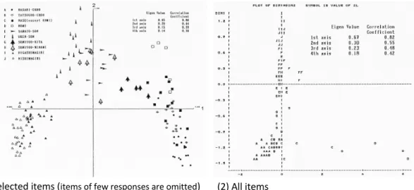
(11) Dialectologia. Special issue, 8 (2019), 117-144. ISSN: 2013-2247. (1) Selected items (items of few responses are omitted). (2) All items. Figure 14. Plot of scores given to localities through Hayashi type 3 (1st axis and 2nd axis).. A multivariate analysis reduces the dimensionality of multidimensional data and demonstrates a simplified structure of the data in a space of lower dimension (Takeuchi et al. 1989: 163, 347). This dimension reduction through multivariate analysis enables the examination of complicated multidimensional data. Inoue (2001: 9, 50) contended that Hayashi’s quantification method type 3 (called Hayashi type 3 for short) was suitable for the processing of nominal scale data originating from linguistic geographical surveys. Figure 14 (Sibata & Kumagai 1993: 487-488) shows some results obtained through the Hayashi type 3 analysis. A simplified structure of the multidimensional LAA data may be noted on a twodimensional space. In Figure 14, a clear distribution of localities corresponding to the dialect divisions of Amami-Ôshima (Figures 7, 8, and 9) may be observed. This output resulted from the processing of the linguistic data without information on the positions of the localities on the geographical space. The analysis depicted an order of geographical distribution in the data. However, because of the dimension reduction, the data processing also caused information loss. A multivariate analysis such as the Hayashi type 3 is optimized to a certain function in multidimensional space in order to group or separate the objects and/or items in the data space.9. 9. The items which have few responses or peculiar localities tend to distort the patterns obtained. Calculating all of the items simultaneously is often not revealing. S&K network method can handle all. 127 ©Universitat de Barcelona.

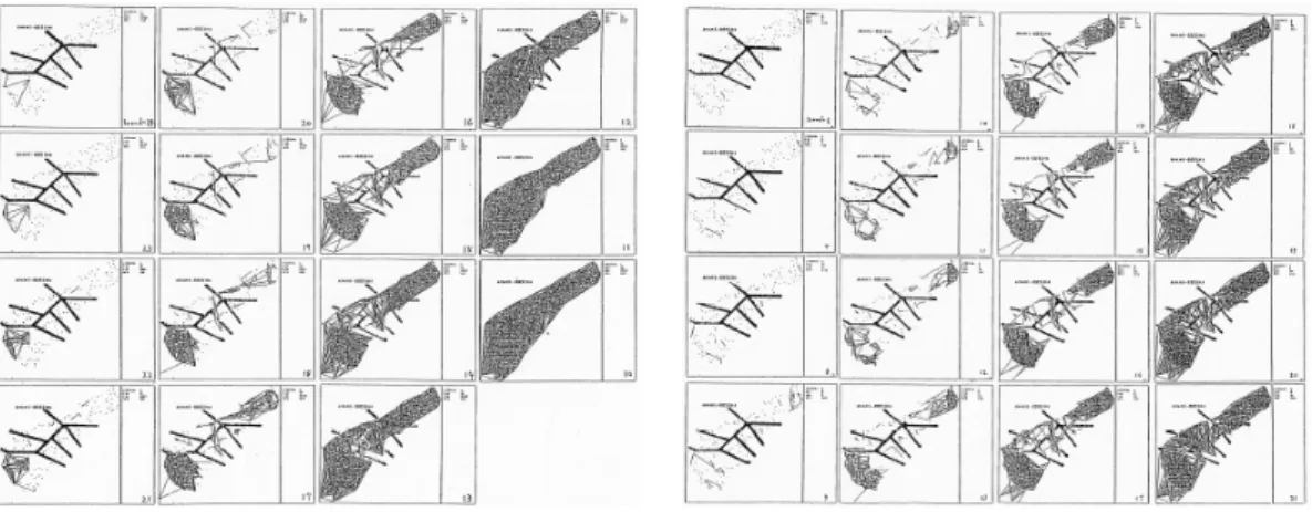
(12) Yasuo KUMAGAI. The S&K network method enables the observation of linguistic similarities among localities on the geographical space without bringing in transformations and relocations concerning the localities in data space. Our data is gathered through a linguistic geographical survey and it encompasses the order of geographical distributions. We aimed to observe the data of this nature without distortion. We (Sibata & Kumagai 1993: 476) compared this feature of the S&K network method to the roles of the scatter diagram in multivariate analyses.10. Figure 15. Geographical distributions of responses and their positions in the scores by Hayashi type 3.. The Hayashi type 3 calculates simultaneous grouping of localities and items.11 Figure 15 depicts sample pictures from a series of distribution patterns, grouped by the results of a cluster analysis (Ward method) to an output of the Hayashi type 3 (Kumagai 2013). The input data comprised all items of the LAA. The geographical the items at the same time and is not disturbed by the number of the responses of each item (Sibata & Kumagai 1993: 467). 10 Recently, spatial statistics is developing. As regards to its application to solve our problem, another consideration will be needed. There are the aspects to be examined from the viewpoint of our purpose. 11 The linguistic features found in a certain lexical form are taken as the items of the input data. The data of LAA is in 1-0 form.. 128 ©Universitat de Barcelona.

(13) Dialectologia. Special issue, 8 (2019), 117-144. ISSN: 2013-2247. distribution of each item and the plots of scores by Hayashi type 3 were put together to grasp the characteristics of this method. Each picture shows a distribution map of a phonological item and three scatter diagrams (the combination of two axes from 1st, 2nd, and 3rd), which exhibits its position (red point) in the plots of all scores of the items as yielded by the Hayashi type 3 analysis. Figures (1), (2), (3) are grouped as the same distribution pattern. Figure (4) belongs to a different group.. 2.5 A formal representation of the continuity of geographical space through the network method. Figure 16. Network representation of NT-1(r)n of Amami-Ôshima.. (1) Delaunay triangulation (2) Delaunay net representation (3) Type 2 representation (4) NT-1(r)n superposed on type 2. Figure 17. Delaunay triangulation and Delaunay net representation of linguistic similarities.. Geographical continuity is an indispensable factor of the S&K network method (Kumagai 1996). The Delaunay triangulation was introduced as a formal representation of geographical continuity to incorporate it into computer processing (Kumagai 1998, 2002, 2013: 4-5, etc.). The Delaunay triangulation is a computational geometrical method of constructing a triangular network that connects adjacent points from randomly distributed points on a plane (Iri & Koshizuka 1993: 126-129). We used this technique as an approximation that represented the continuity of geographical space. 129 ©Universitat de Barcelona.

(14) Yasuo KUMAGAI. Figure 17 (1) shows the Delaunay triangulation of Amami-Ôshima island. In order to observe linguistic similarities among localities along geographical spaces, we assigned a value of linguistic similarity NC (or DC) to a line connecting two adjacent points of the Delaunay network to visualize the varying degrees of linguistic similarity among the localities (Figure 17 (2)). Figure 17 (3) is its type 2 representation evincing higher values of NC on lesser line-width. We named this configuration the Delaunay net representation. In Figure 17 (4), NT-1(r)n (Lcond=17 in Figure 16) is superposed on Delaunay net type 2. This network is an approximation and it does not represent continuity based on the actual contact between people, reflecting human communication. This representation was utilized as a tool to observe our data along a path of geographical continuity. Therefore, it must be noted that localities connected by lines on the Delaunay net do not necessarily indicate the existence of human contact between the localities. A link that depicts high degrees of likeness on the Delaunay net representation does not necessarily indicate close contact between people in those areas. The actual knowledge of the real world must be acquired to properly utilize this network representation.. 3. Development and utilization of the Linguistic Atlas of Japan Database. Figure 18. A map from the LAJ (to be, to exist).. 130 ©Universitat de Barcelona. Figure 19. A map from the LAJ (heel)..

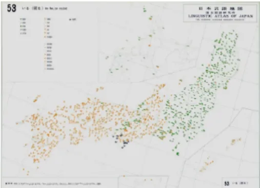
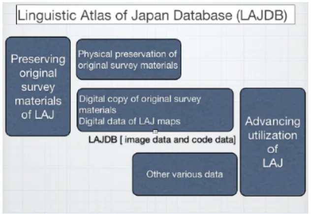
(15) Dialectologia. Special issue, 8 (2019), 117-144. ISSN: 2013-2247. Figure 20. The framework of the LAJDB project.. Figure 21. Factors related to the LAJDB.. Figure 22. A snapshot of image database. Figure 23. A snapshot of coded data.. The Linguistic Atlas of Japan (NLRI 1966-1974, 6 volumes) or the LAJ in short, was the first nationwide linguistic atlas in Japan that was based on the linguistic geographical survey method (2,400 localities surveyed from 1957 to 1965, Figures 18 and 19). This survey was conducted by the National Language Research Institute (NLRI, currently National Institute for Japanese Language and Linguistics: NINJAL). Sibata and Grootaers both functioned in distinguished roles in this project. Sibata headed the section responsible for the survey during the entirety of the survey period (from 1955 to 1964); Grootaers played an important part in the project from the beginning of the survey to its publication.12 After its publication, the LAJ became an important research resource for dialectology. However, the acquisition of digital data pertaining to the LAJ was impossible in those days. 12. Grootaers influenced dialect geographical studies since his arrival in Japan (NLRI 1966, Appendix A: 46).. 131 ©Universitat de Barcelona.

(16) Yasuo KUMAGAI. The development of the Linguistic Atlas of Japan Database (LAJDB) began in 1999. This digitalized version attempts to render the entire information of the LAJ digitally to make it available on computers (Kumagai 2016: 334-338). The LAJDB aims to preserve the original survey materials (540,000 cards) through digitization and promote the advancement of the multiple utilities of the LAJ (Figures 20, 21). The LAJDB comprises an image database of the original survey materials (Figure 22) and encompasses coded data corresponding to the published maps (Figure 23). Hereafter, the terms LAJDB55, LAJDB42,13 and GDF (Geographical Distribution of Frequency) will be used in this paper for easier reporting.. Figure 24. Standard form (△) and NEW by speakers (▲).. (1) Usage rate by prefecture. Figure 25. GDF of NEW by speakers.. (2) GDF of standard forms. Figure 26. Frequency of standard forms.. Figure 27. Network representation on Delaunay net (NC).. 13. LAJDB55 is a subset of the LAJDB in progress. The number of surveyed localities was not equal for each item. It consists of 55 items from LAJDB with 2400 ± 1 localities. LAJDB42 is a subset of LAJDB55 to explore the distribution of the standard forms. Two or more forms were occasionally recognized as standard by the LAJ’s editors. The LAJDB42 consists of 42 items with unique standard forms.. 132 ©Universitat de Barcelona.

(17) Dialectologia. Special issue, 8 (2019), 117-144. ISSN: 2013-2247. The LAJ surveyed 2400 localities nationwide. This quantity enables the precise imaging of countrywide associations pertaining to dialect distributions and extralinguistic factors. Further, the original survey card images linked to each entry of coded data enable access to the original phonetic recordings, the comments of informants (speakers) and the notes inscribed by the fieldworkers and editors. This accessibility to the original survey materials accords the ability to trace the categorization of the word forms registered on the LAJ. It also affords access to the original transcriptions made by the fieldworkers, the remarks made by the informants (speakers), as well as notes inscribed by the fieldworkers, which are not available in the published LAJ. Figures 24 and 25 show such examples of the utilization of the NEW of the standard forms of the informants’ comments (“This is a new polite form”, etc.) from inscriptions made on the original survey cards. Figure 26 and 27 are some examples of the utilities of the compilation of precise nationwide data from 2400 localities. Figure 26 (1), based on the data obtained from Kasai,14 evinces the usage rates of the standard forms summarized by prefecture, prepared through a manual reading the LAJ maps. Figures 26 (2), based on LAJDB, demonstrates a precise nationwide picture of the frequency distribution by locality that could not be depicted by former studies using the paper printed LAJ. Figure 27 is an example of the Delaunay net representation showing a nationwide representation of linguistic similarities.. Figure 28. Some maps of extra-linguistic factors of LAJ (Introductory maps I, II, V).. Figure 28 displays some examples from the LAJ of the maps of extra-linguistic factors. These illustrations were intended for the interpretation and analyses of dialect 14. Kasai, Hisako (1981) “Hyôjun gokei no zenkoku bunpu” [Nationwide distribution of standard forms], Gengo seikatsu, 354, 52-54.. 133 ©Universitat de Barcelona.

(18) Yasuo KUMAGAI. distributions. These have been transformed into some digital maps, including (a) the basic map of LAJ, (b) a topographical map showing mountain systems, river systems, etc., (c) main roads that existed in the Meiji period (approximately 1885) and (d) the boundaries of the feudal domains during the Edo period (1664) (Kumagai 2016: 338). Further, we have added digital data of historical maps on which map (c) is based, population maps, time series population data, and so on.15 In conjunction with the data pertaining to the extra-linguistic factors and other various publicly opened data, the LAJDB enables the detailed observation of the relationships between dialect distributions and extra-linguistic factors.. 4. People, contact, network, and geographical space. 4.1 Network of linguistic similarities and population distribution. Figure 29. Delaunay net of linguistic similarities (NC) and population distribution.. 15. The time series population data of the National Census from 1920 to 1980, adjusted on the basis of the boundaries of the 3433 municipalities at the time of the 1980, for the time series comparisons is based on “Toyo Keizai Shinposha (ed.). 1985. Population statistics of Japan: Summary of National Census & other surveys, 1872 -1984. Tokyo: Toyo Keizai Shinposya.”. 134 ©Universitat de Barcelona.

(19) Dialectologia. Special issue, 8 (2019), 117-144. ISSN: 2013-2247. Figure 29 displays a series of maps obtained by the superposition of the Delaunay net (LAJDB55 data) of different opacities on the population distribution of 1960. The population of each municipality (municipal boundary: 1980) is plotted at the place of its office.16 A similar pattern may be noted between the network of linguistic similarities and the population distribution. 4.2 Population distributions, road networks and municipal boundaries. Figure 30. Population distribution (National census 1955) and road network.. Figures 30 (1) and (2) display the main roads around 1885 and the present-day road network17 superposed on the population distribution and the density according to municipalities 18 (national census 1955). These figures reveal the correspondence between densely populated areas and regions with highly developed road networks.. Figure 31. Changes in Population.. Figure 32. Changes in population by prefecture.. 16. Each red disk which denotes population size (9 categories) is in the proportion size of each municipality. 17 Road network data of present day: Geospatial Information Authority of Japan (2011); Global Map Japan in Global Map ver. 2.0. 18 Geographical Survey Institute and Statistic Bureau of Ministry of Internal Affairs and Communications (1958) Population distribution and density by shi machi mura: Population census of 1955, Geographical Survey Institute.. 135 ©Universitat de Barcelona.

(20) Yasuo KUMAGAI. Figure 33. Changes in population distribution superposed on road network (central Japan).. Figure 34. Changes in number and boundary19 of municipalities.. Figures 31-33 evince the changes in population: the increase in population, the substantial growth of the metropolitan areas, and their expansion. However, the population distribution pattern remains relatively stable. Although the numbers and boundaries also change (Figures 34), the distribution patterns of the density of municipalities are relatively constant and correspond to the population distributions (Figure 28(2), 29(6)).. 19. Boundary data: Restored previous municipal boundaries, Administrative boundary data of Taisho and Showa Era (Y. Murayama lab. Tsukuba University).. 136 ©Universitat de Barcelona.

(21) Dialectologia. Special issue, 8 (2019), 117-144. ISSN: 2013-2247. 4.3 Observing phenomena related to dialect distributions on geographical space. Figure 35. The GDF of standard forms and the road network.. Figure 36. The GDF of multiple answers (MA) and population distribution.. Figure 37. The GDF of the NEW of standard forms and population distribution.. 137 ©Universitat de Barcelona.

(22) Yasuo KUMAGAI. Figure 35 exhibits the correspondence between the GDF of standard forms and areas of developed road networks. Figure 36 shows the GDF of multiple answers and the population distribution and Figure 37 displays the GDF of the NEW of standard forms and the population distribution. These figures reveal the significant mutual correspondences from the viewpoint of diffusions, e.g., the different correspondents of distribution patterns among them depending on the locations such as the Tokyo area (present center), the Kyoto area (old center) and the regions connecting them.. Figure 38. The GDS, population distribution, and road network (two examples from 2400).. Geographical distributions of the degrees of similarity (GDS) from a reference point is superposed on (2) the population distribution and (3) the road network. The correspondence of the GDS is observed with regard to the population distribution and the road network both in A and in B.. 138 ©Universitat de Barcelona.

(23) Dialectologia. Special issue, 8 (2019), 117-144. ISSN: 2013-2247. Figure 39 Main roads, municipal boundary, population distribution and Delaunay net linguistic similarity.. Figure 39 displays the main roads (around 1885) superposed on (1) the municipal boundary, (2) the population distribution and the municipal boundary, and (3) the Delaunay net representation of linguistic similarity. These are significantly related.. 5. Concluding remarks Grootaers (1976: iv) posited that the discovery of the “relations of human and ‘space and time’, which are deeply intertwined in unconscious way”, was one of the focal issues for linguistic geographical studies. The observations made above evince repeatedly appearing patterns, both linguistic and extra-linguistic. These patterns exhibit significant relationships, which are supposed to reflect human communication and the social life of the communities in geographical space; they also reveal the cumulative effects of the historical process of these factors (Figure 40).. 139 ©Universitat de Barcelona.

(24) Yasuo KUMAGAI. Figure 40. Mutually related factors and observations on which this paper focused.. Chikio Hayashi (1918-2002), a pioneer of data science in Japan, indicated the existence of two positions in data analysis: that which functions as a probe to explore data to draw useful knowledge, and that which acts as a pointer to directly mark what we want to know. He named these positions the first word and the last word of data analysis, respectively. Each consists of different characteristics and should not be confused in creations and applications of the methods of data analysis. (Hayashi et al. 1970:2-5). The observations tendered above intended to view the available data from multiple perspectives and to grasp the nature of the data through the intention to discover phenomena. The first word of data analysis is important and must be executed carefully. More precise scrutiny needs data to be integrated, and this task is currently being undertaken. In 1948, Sibata participated in a nationwide social survey entitled the Literacy Research of Japan. This well-known statistical survey was the first to use the random sampling method in Japan. Sibata met Chikio Hayashi during this project. After the survey, Sibata joined NLRI in 1949 and conducted a series of surveys on the linguistic life of the Japanese (Japanese sociolinguistics) using scientific approaches such as statistical methods. After the sociolinguistic studies including the standardization of regional societies, Sibata engaged in the LAJ survey. He wrote that his encounter with linguistic geography helped him overcome a one-sided view of language, whether synchronic or diachronic. According to him, linguistic geography is the scientific method of analyzing languages in rapport with each other (Sibata 1969: 3-4). His linguistic geography. 140 ©Universitat de Barcelona.

(25) Dialectologia. Special issue, 8 (2019), 117-144. ISSN: 2013-2247. became real after his meeting with Grootaers. They became very good friends and maintained a lifelong collaboration (Sibata 1988a, 1990, 1995). I studied linguistics under Sibata at Saitama University (1979-1984). Sibata evinced his respect for ordinary people. He emphasized the importance of philosophy in scientific studies. Grootaers and Sibata shared a common spirit with regard to the study of language: linguistics is the study of human language. Sibata insisted that “Language changes. However, it does not change naturally. It is human that changes language”. The two scholars never forgot the people who spoke the language they studied. The development and analysis of data go hand in hand. The construction of the LAJDB and the diverse data concerning external factors led to the enrichment of the LAJ as a research resource and caused the extension of further research potential. The concept of a network is fundamental to the S&K network method. Thinking about a network is also thinking about contact. Distributions of dialects, speech communities and dialect areas are all networks and they are developed through contact between people who inhabit expanses of land. The development of the S&K network method and the LAJDB are both motivated by their common spirit of linguistic studies.. Acknowledgments LAJDB was supported by a Grant-in-Aid for Publication of Scientific Research Results (database) in 2001, 2002, 2003, 2004, 2005, and 2008 (Project Leader: Yasuo Kumagai). This paper includes some outcomes of the collaborative research projects “Analyzing large-scale dialectal survey data from multiple perspectives” (2009-2012, Project Leader: Yasuo Kumagai), “General Research for the Study and Conservation of Endangered Dialects in Japan” (20132015, Project Leader: Nobuko Kibe), “Endangered Languages and Dialects in Japan”(2016-, Project Leader: Nobuko Kibe) at the National Institute for Japanese Language and Linguistics; and “Development of quantitative methods of analyzing large-scale dialectal distribution data” (Grants-in-aid for scientific research, JSPS KAKENHI Grant Number 26370555, 2014-2017, Project Leader: Yasuo Kumagai). I thank prof. Chitsuko Fukushima for her comments.. 141 ©Universitat de Barcelona.

(26) Yasuo KUMAGAI. References GROOTAERS, Willem A. (1976) Nihon no hôgen chirigaku no tame ni [Studies of Japanese linguistic geography], Tokyo: Heibonsha. HAYASHI, Chikio, Isao HIGUCHI & Isamu KOMAZAWA (1970) Jôhôshori to tôkeisûri [Information processing and statistical mathematics], Tokyo: Sangyo tosho. INOUE, Fumio (2001) Keiryôteki hôgen kukaku [Quantitative dialect division], Tokyo: Meiji shoin. IRI, Masao & Takashi KOSHIZUKA (eds.) (1993) Keisan kikagaku to chiri jôhôshori [Computational geometry and geographical information processing], 2nd ed., Tokyo: Kyoritsu shuppan. KATO, Masanobu (1977) “Hôgenkukakuron” [Studies of dialect division], in Iwanami kôza Nihongo 11 Hôgen, Tokyo: Iwanami shoten, 41-82. KOKURITSU KOKUGO KENKYÛJO (NLRI) (1966-1974) Nihon gengo chizu [Linguistic atlas of Japan], 6 vols., Tokyo: Printing bureau, Ministry of Finance. KUMAGAI, Yasuo (1996) “Hôgen kukaku no hôhô ni okeru chiriteki na jigen” [Geographical dimension in the methods for dividing dialect area], in Gengogakurin 1995-1996 henshû iinkai (ed.), Gengogakurin 1995-1996, Tokyo: Sanseido, 1209-1219. KUMAGAI, Yasuo (1998) “Nihongengochizu dai 3 shû no nettowâku ni yoru chitenkan ruijido hyôji to chikei zinkô bunpu jôhô to no kasaneawase” [Superposition of network representation of linguistic similarities among localities, topography and population distribution: Linguistic Atlas of Japan volume 3 data], Conference papers of the dialectological circle of Japan, 66, 49-56. KUMAGAI, Yasuo (2002) “Keiryôteki hôgen kukaku to hôgen chirigaku: Keiryôteki hôgen kukaku no tame no Nettowâkuhô no kaihatsu o tôsi te” [Quantitative dialect division and dialect geography: Development of S&K network method], in Yoshio Mase (ed.), Hôgen chirigaku no kadai, Tokyo: Meiji shoin, 150-164. KUMAGAI, Yasuo (2013) “Development of a Way to Visualize and Observe Linguistic Similarities on a Linguistic Atlas”, Working Papers from NWAV Asia-Pacific 2, 1-8. <https://pj.ninjal.ac.jp/socioling/nwavap02/Kumagai-NWAVAP2-2013.pdf> KUMAGAI, Yasuo (2016) “Developing Linguistic Atlas of Japan Database and advancing analysis of geographical distributions of dialects”, in Marie-Hélène Côté, Remco Knooihuizen & John Nerbonne (eds.), The future of dialects: Selected papers from Methods in Dialectology XV, Berlin: Language Science Press, 333-362. <http://langsci-press.org/catalog/view/81/159/390-1] > [DOI:10.17169/langsci.b81.159]. 142 ©Universitat de Barcelona.

(27) Dialectologia. Special issue, 8 (2019), 117-144. ISSN: 2013-2247. KUMAGAI, Yasuo & Takesi SIBATA (1987) “Gengoteki tokuchô ni yoru chiikibunkatsu no tame no Nettowâkuhô II: Nettowâkuhô to ta no hôhô to no hikaku o chûshin ni” [The Network method for dividing dialect area on the basis of linguistic features (2): Focusing on comparisons with other methods], Conference papers of the dialectological circle of Japan, 44, 57-65. NLRI. See Kokuritsu Kokugo Kenkyûjo (NLRI). SIBATA, Takesi (1964) “Hôgenkukaku to wa nani ka” [What is dialect division?], in Nihon hôgen kenkyûkai (ed), Nihon no hôgen kukaku [Dialect division of Japan], Tokyo: Tokyodo, 5-22. SIBATA, Takesi (1969) Gengochirigaku no hôhô [Method of linguistic geography], Tokyo: Chikumashobo. SIBATA, Takesi (1978) Shakaigengogaku no kadai [Issues of sociolinguistics], Tokyo: Sanseido. (English translation: Takeshi Sibata; ed. by Tetsuya Kunihiro et al. (1999). Sociolinguistics in Japanese contexts, Berlin: Mouton de Gruyter.) SIBATA, Takesi (1982a) “Amami-Ôshima no hôgen kukaku” [Dialect boundaries in the AmamiÔshima Island], in Kyûgakkai rengô Amami chôsa iinkai (ed), Amami: shizen, bunka, shakai, Tokyo: Koubundou, 150-156. SIBATA, Takesi (1982b) “Shima to sono kotoba” [Island and its language], Gengo seikatsu, 368, 18-26. SIBATA, Takesi (ed.) (1984) Amami-Ôshima no kotoba: Bunpu kara rekisi e [Language of AmamiÔshima: from distribution to history], Musashino: Akiyama shoten. SIBATA, Takesi (1988a, 1990, 1995) Itoigawa gengo chizu 1, 2, 3 [Linguistic Atlas of Itoigawa 1, 2, 3], Musashino: Akiyama shoten. SIBATA, Takesi (1988b) Hôgenron [Dialect studies], Tokyo:Heibonsha. SIBATA, Takesi & Yasuo KUMAGAI (1984) “Gengoteki tokuchô ni yoru chiiki bunkatsu no tame no "Nettowâkuhô"” [The Network method for dividing dialect area on the basis of linguistic features], Conference papers of the dialectological circle of Japan, 38, 45-63. SIBATA, Takesi & Yasuo KUMAGAI (1985) “Gengoteki tokuchô ni yoru chiiki bunkatsu no tame no "Nettowâkuhô": Toku ni NT-1(r) ni tsuite” [The “Network method,” a method for dividing an area on the basis of linguistic features: With a special reference to NT-1(r)], Kokugogaku, 140, left 45-60. SIBATA, Takesi & Yasuo KUMAGAI (1987) “Nettowâkuhô ni okeru chitenkan no gengoteki ruizi no atarashii toraekata to shori no shikata: Gengoteki tokuchô ni yoru chiiki bunkatsu no. 143 ©Universitat de Barcelona.

(28) Yasuo KUMAGAI. tame no Nettowâkuhô II” [A new "Network method" and its processing procedures for dividing dialect areas], Kokugogaku, 150, left 1-14. SIBATA, Takesi & Yasuo KUMAGAI (1993) “The S&K network Method: Processing Procedures for Dividing Dialect Areas”, Zeitschrift für Dialectologie und Linguistik, 74, 458-495. TAKEUCHI, Kei et al. (eds.) (1989) Tôkeigaku jiten [A dictionary of statistics], Tokyo: Toyo keizai shinposha.. 144 ©Universitat de Barcelona.

(29)