NOTE ON STABILITY OF AN SIRS EPIDEMIC MODEL (Theory of Biomathematics and Its Applications XII : Mathematical and experimental approach to clarify patterns in a transition process)

NOTE ON STABILITY OF AN SIRS EPIDEMIC MODEL

YUKIHIKO NAKATA

ABSTRACT. Inthis paperwederive ascalardelaydifferentialequationfrom.an

epidemic model with waning immunity. The model is formulated asa system

of delay differential equations. The characteristic equation is computed. We

visualizethestabilitycondition foranendemic equilibrium inatwo-parametcr

plane.

1. INTRODUCTION

In [9] we consider periodicoutbreak ofmycoplasma pneumoniacin Japan. Minor

variation of the immunity period is shown to be essential in order to explain the infectious disease dynamics. Ouragendaincludes mathematical studie$s^{}$ $\{\dot{o}r$periodic

solutions of the mathematical model employed in [9]. This note is

a

prcliminary study for the project. The modelin $|9$] takes theform ofSEIRStype epidemic model with a gamma distribution which thc immunity period follows. In this papcr for mathematical analysis we consider SIRS type epidemic model with fixed immunity

period (such that the variance of thc immunc period is zero). Let us consider thc following SIRS epidcmic model

(l.la) $\frac{d}{dt}S(t)=-\beta S(t)I(t)+\gamma I(t-\tau)$,

(l.lb) $\frac{d}{dt}I(t)=\beta S(t)I(t)-\gamma I(t)$,

(l.lc) $\frac{d}{dt}R(t)=\gamma I(t)-\gamma I(t-\tau)$,

where the total population is fixed as

(1.2) $S(t)+I(t)+R(t)=1, t\geq-\tau$

and recovered population satisfies

(1.3) $R(t)= \gamma\int_{0}^{ア}I(t-s)ds, t\geq 0.$

Here $S(t)$, $I(t)$ _and $R(t)$ respectively denote the fraction of susceptible, infectivc

and recoveredpopulations at time$t$

.

The model has threeparameters: transmission

coefficient $\beta>0$, the recovery rate $\gamma>0$ and the imrnunc period $\tau>0$. We also

refer the papers [6, 10, 4] for analyses of similar SIRS epidemic znodels. See also

{5]

for detail of compartmental modcl inepidemiology. The model (1.1) appears in the paper $|5$] and we here $revie\backslash v$ thc stability analysis.

From (1.2) and (1.3)

we

get

$S(t)=1-I(t)- \gamma\int_{0}^{ア}I(t-s)d_{\mathcal{S}}$

then we obtain a scalar delay differential equation:

(1.4) $\frac{d}{dt}I(t)=I(t)\{\beta(1-I(t)-\gamma\prime_{0^{\gamma}}J(t-s)ds)-\gamma\}.$

The basic reproduction number is given as $R_{4}:= \frac{\beta}{\gamma}.$

It is assumed that $R_{0}>1$ holds

so

that (1.4) has

a

positive equilibrium:

$I_{e}:= \frac{1-\frac{1}{R_{0}}}{1+\gamma\tau}.$

Remark 1. $\gamma\tau=-\frac{\tau r}{\gamma}$ denotes the fraction of the immunity period

over

the expected

infectious period, which may be

a

large parameter. Note that

$\gamma_{\mathcal{T}>}1rightarrow\tau>\frac{1}{\gamma}$

implies that the immunity period is longer than thc expected infectious period.

We normalize the equation (1.4) defining

$x(t):= \frac{I(t\rangle}{I_{e}}-1$

and $su\})$scqucntly consider the $nondimcnsiol\backslash al$ tinxe $u= \frac{t}{\tau}$. Abusing notation we

finally obtain

$(1.5\rangle$ $\frac{d}{dt}x(t)=-p(x(t)+1)(x(\ell_{j})+\eta\int_{()}^{1}x(t-s)ds)$ ,

where

(1.6a) $p:= \frac{\gamma\tau}{1+\gamma\tau}(R_{\zeta)}-1)\}$

(1.6b) $\eta:=\gamma\tau.$

Initial condition for (1.5) is

$x(\theta)=\psi(\theta)\geq-1, \theta\in[-1, 0],$

excluding $tl\backslash c$ constant function _{$\psi(\theta)\equiv-1,$ $\theta\in[-1, 0].$}

Remark 2. To apply the time transformation

wc

introduce a nondimensional timc $u= \frac{t}{r}$ and define

$\tilde{x}(u):=\tilde{x}(\frac{t}{\tau})=x(t)$.

Tlzen olae can

see

$\frac{d}{du}\tilde{x}(u)=\tau\frac{d}{dt}x(t)$ and

NOTE ON STABILITY OF AN SIRS EPIDEMIC MODEL

2. STABILITY ANALYSIS

Applying the fluctuation lemma we can obtain a global stability result. There

seems

to be

no

other results for global stability. See also the global stability

condi-tion by the fluctuacondi-tion lemma in $|7$].

Theorem 3. Let

us assume

that $\eta<1$ holds. Then the trivial equilibrium

of

(1.5)

is globally attractive.

Proof

Lct us writc

$\overline{x}=\lim\sup x(t) , \underline{x}=\lim_{tarrow}\inf_{\infty}x(t)$.

$tarrow\infty$

Consider a sequence such that $x(t_{n})arrow\overline{x}$

as

$narrow\infty$ with $x’(t_{n})\geq 0$

.

Then

we

get $0 \geq x(t_{n})+\eta\int_{0}^{1}x(t_{n}-s)ds.$

Taking the limit and estimating the second term ofthe right hand side from below

by $\underline{x}$, we get

$0\geq\overline{x}+\eta\underline{x}.$

Similarly, considering a sequence which tends to $\underline{x}$, we get

$0 \leq x(u_{71})+\eta\int_{0}^{1}x(u_{n}-s)ds.$ Thus $0\leq\underline{x}+\eta\overline{x}.$ Therefore it holds $\overline{x}+\eta\underline{x}\leq 0\leq\underline{x}+\eta\overline{x},$ thus $(\overline{x}-\underline{x})\leq\eta(\overline{x}-\underline{x})$ .

Since $\eta<1$ is assumed, we obtain $\underline{x}=\overline{x}$. It is easy to

see

that $\underline{x}=\overline{x}=0$

follows. $\square$

If $\eta<1$ then $t$he trivial equilibrium is shown to be asymptoticaJly stable in thc

following section.

2.1. Linearized stability analysis. To analyze asymptotic stability of thc

triv-ial equilibrium of (1.5) we derive the characteristic equation. The characteristic

equation is computed as

(2.1) $\lambda=-p(1+\eta\int_{0}^{1}e^{-\lambda s}ds) , \lambda\in \mathbb{C}.$

We $al)$alyzc the characteristic equation (2.1) following Chapter XI of $|2$]. See aJso

[3, 1, 8] for analysis of characteristic equationsof dclay equations. One

can

$\sec$ that

$\lambda=0$ is a root of (2.1) if$p=0$ holds, where the transcritical bifurcation

occurs

(as

$p$ increases). Substituting $\lambda=i\omega,$ $\omega\in \mathbb{R}$ we gct

(2.2) $0=1+ \eta\int_{0}^{1}\cos(\omega s)ds,$

$R\sim om(2.2)$

one

has

$\eta=\frac{-1}{\int_{0}^{1}\cos(\omega s)ds}=-\frac{\omega}{\sin\omega}.$

Thcn$p$ is determined from (2.3) as

$p= \frac{\omega}{\eta\int_{0}^{1}\sin(\omega s)ds}=-\frac{\omega\sin\omega}{1-\cos\omega}.$

For $n\in N_{+}$ let

$I_{n} :=((2n+1)\pi, 2(n+1)\pi)$.

Thc parametric curve

(2.4) $( \eta(\omega), p(\omega))=(-\frac{\omega}{si_{11}\omega}\prime-\frac{\omega si_{12}\omega}{1-\mathfrak{c}\cdot.os\omega}) \omega\epsilon I_{n}.$

depicts the condition whcre the characteristic equation (2.1) has

a

conjugated pair

of pul’cly imaginary roots $\lambda=\pm i\omega,$ $\omega\in I_{n}$

.

One

can

easily

see

that $(\eta(\omega)_{:}p(\omega)\rangle\in \mathbb{R}_{+}^{2}, \omega\in I_{7?}.$

The parametric

curve

(2.4) can be trarslated in terms of $R_{0}$ and $\gamma\tau$ using the

relation (1.6). Wc get tluc following condition

$R_{0}-1=- \frac{\omega\sin\omega}{1-\cos\omega}(1-\frac{\sin\omega}{\zeta_{4}\}})$ ,

$\gamma\tau=-\frac{\omega}{si_{11}\omega},$

$\backslash \backslash$here the charactcristic equation (2.1) has purely

$i_{1}$naginary roots.

3. $DlSC($jSSION

We here sketch the stability allal$\backslash$/sis ノ for the SIRS epidemic model with delay.

Although the $modc!1$ _{equation has} a simple looking, it exhibits destabilization of

the cndemic equilibrium and has a periodic solutions via Hopf bifurcation. In the paper $|9$] wc discuss a role of the minor variation of thc $i\iota$nxnunity period in thc

periodic cpidclnic cycle sccll in a childhood disease, in particular, for small $R_{0}$. Sce

also $\zeta 8$]. The author study periodicity and uniqucllcss of a periodic solution $oi$

.

thc

equation (1.5) in the collaboration with G. Kiss, _{G. Vas and R.} Omori.

Acknowledgment. Thc author $\iota vas$ supported $b$ JSPS Fellows, No.268448 of

Japan Society for the Promotion of Science. A part of $t1_{1}is$ paper is written during

thc stay at thc Bolyai Institute of thc Univcrsity ofSzeged in February 2016. The research visiting was supported by JSPS Bilatcral Joint Rcscarch Project (Open Partnership).

REFERENCES

$|$1} T. Alarc\’o11, Ph. Getto,y. Nakata, Stability analysis of a rcncwalequationfor cell population

dynamics With quicsccnce. SIAM J. Appl. Math. $\sim(4$ (4$\rangle$ pp. 1266-1297 (2014)

[2] $\circ$. Dickmann, S.A. van Gils, S.M.y. Lunel. H.-O. Walthcr, Delay Equations FUnctiona],

Complex and Nonlinear Analysis, Springcr Vcrlag (1991)

$|$3$|$ O. Dickmann, Ph. Getto, y. Nakata, On thc characteristic equation$\lambda=\alpha 1+(\alpha_{2}+\alpha 3\lambda)e^{-\lambda}$

and its use in the context ofa cell population model. J. Math. Bio. 72 (4) pp 877-908 (2016$\rangle$

[4] S. Gongalves, A. Guillermo, M.F.C. Gomcs Oscillations in SIRS model with distributed

dc-lays. TheEuropean Physical Journal $B$-Condensed Mattcr and Complex Systems, 81(3) pp.

NOTE ON STABILITY OF AN SIRS EPIDEMIC MODEL

$\eta$

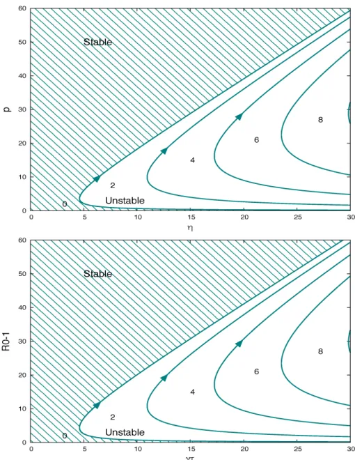
FIGURE 2.1. Stability boundary of the endemic equilibrium in

$(\eta,$p) planc (above) and in $(\gamma\tau, R_{0}-1)$ plane (below). The number

depicts the number of roots of the characteristic equation in the

right half complex plane. Thc arrows in the curves indicate the

direction ofincreasing $\omega.$

[5] H.W. Hethcotc, H.W. Stech, P. van dcnDriesschc, Nonlinear oscillationsin cpidcmicmodels.

SIAM J. Appl. Math., 40 pp. 1-9 (1981)

[6] Y.N. Kyrychko, K.B. Blyuss, Global properties of a delayed SIR model with temporary

immunity and nonlincar incidence rate. Nonlinear Anal. RWA. 6 pp. 187-204 (2005)

[7]y. Nakata, Y. Enatsu, H. Inaba, ’r. Kuniya, Y. Muroya, Y. Takcuchi, Stability ofepidemic

models with waning immunity. SUT J. Math. 50 (2) 205-245 (2014)

[8] Y. Nakata, R. Omori, Delay equationformulation foran epidemic model with waning

immu-nity: an application to mycoplasma pneumoniae. IFAC-PapersOnLine 48 (1S) pp. 132-135

[9] R. Omori,Y. Nakata, H.L.Tcssmer, S. Suzuki, K. Shibayama,The determinant ofpcriodicity

in Mycoplasma pneumoniae incidence: an insight from mathematical modelling. Scientific

Reports _5: 14473 (2015)

[10] M.L. Taylor, T.W. Carr, An SIR epidemic modc}with partial temporary immunity modeled with delay. J. Math. Bio. 59 (6) pp. S41-S80 (2009)

GRADUATE SCHOOL 0F $MATH\otimes$MATlCAL SCIENCgS, TME $UNlVBRS\ddagger TY$ _0F $ToKYO_{{\}}$ 3-8-1,