渦管の3次元不安定性再考 (非線形波動現象の構造と力学)

渦管の

3

次元不安定性再考

九大数理 福本 康秀

(Yasuhide Fukumoto)

Graduate School of

Mathematics,

Kyushu University

概要 3 次元流中において 1 本の渦管に着目したとき, まわりの渦や背景流の影響は, まず 移流として, 次にその渦管の中心線上の各点を原点とする局所線形ひずみ流として近似的 にとりこむことができよう. 渦度に垂直な断面内に速度成分をもつ 2 次元純粋ずり流中 におかれたまっすぐな渦管は 3 次元撹乱に対して線形不安定であることが, 単純な設定 のもとで Widnall 等によって具体的に明らかにされた 1). Widnall 不安定’ はそれ以後の 渦管の安定性の議論における中心をなす

:

局所純粋ずり流によって断面がわずかに楕円形に変形した渦柱を基本流にとる. 断面 が円形の渦は中立安定である. とくに, 渦度分布が一様のものが ‘Rankine の渦’ で, そ の上に立つ無限個の固有振動モードは ‘Kelvin 波’ とよばれる. 渦度ベクトルに垂直な断

面 (x 架平面) 上に渦中心を原点とする極座標 $(r, \theta)$ を導入しよう. 純粋ずり流は $\cos 2\theta$ と

sin20 によって特徴づけられる. いわゆる, ‘四重極子’ 流である. この四重極子場を介し

て, Kelvin 波のうちの右巻き・左巻きの屈曲モード ($e^{\dot{|}\theta}$, $e^{-\dot{|}\theta}$

成分) が共鳴を起こして指 数関数的に成長する, というのがそのシナリオである. 本研究では, Widnall 不安定’ をハミルトンカ学系におけるスペクトル理論の枠組み に乗せ, これを別の側面から眺めてみる. Krein の理論によると, 単独の Kelvin モード に微小摂動を加えても不安定化することはなく, 少なくとも 2 個のモードの波数 $k$ と周 波数 $\omega$ が一致して始めて不安定化が可能になる. すなわち, $(k, \omega)$ 平面上に描かれた分 散関係を表す ₂ 木, もしくはそれ以上の, 曲線が交差しなければならない. 円形渦に対す

る摂動が四重極子流である場合には, $e^{\dot{|}m\theta}$, $e^{\dot{|}n\theta}$ 型の角度依存性をもつ 2 つの Kelvin モー

ドが, 関係 _$|m-n|=2$ を満たすときに限って, 分散曲線の交点上で共鳴を起こし得る.

実際, ₂ つの屈曲モード $m=1$ と $n=-1$ はこの条件を満たしている. しかし, 分散曲

線が交差すればいつでも不安定化するというわけではない. 攪乱がもつエネルギーの符号

が問題で, 同符号のエネルギーをもつ攪乱同士では不安化は起こり得ず, 片方の攪乱のエ

ネルギーが正で他方が負であることが共鳴不安定のための必要条件である.

さて, Widnall&Tsai (J. Fluid Mech. 1976) での固有値・固有関数の表式は不定積

分を残したままになっており, 当時の数値計算では十分な精度が得られなかったようで ある. 実はこの積分は実行できて線形安定性問題の解が Bessel 関数を用いてあらわに書 き下せることに気づいた. 固有値・固有関数の高精度数値計算をもとに Widnall&Tsai (1976) の不備を修復し, さらに, Widnall 不安定’ と‘楕円型不安定’ との関係について 検討を加える (\S 4). 屈曲波の分散曲線の交点上で必ずパラメータ共鳴不安定が起こる. Kelvin 波のエネル ギーの計算を実行し, この結果が _Krein 理論と矛盾しないことを示す (\S 5). これらの結果の要約については FukumotO&Hattori (2002 も参照されたい. 数理解析研究所講究録 1271 巻 2002 年 210-219

210

1Introduction

Moore

&Saffman

(1975) and Tsai

&Widnall

(1976), hereinafter being referred to as MS75 and TW76 respectively, addressed athree-dimensional linear stability problem of

a

straight vortex tubeembeddedin aplane pureshearflowwith its principalaxes

perpendic-ular to thetubeaxis, anduncovered theessence ofaparametricresonancebetween the left-and right-hleft-anded helical

waves

driven by the imposed shear. The

Moore-Saffman-Tsai-Widnall instability is rather successfully adapted to

an

explanation for the short-wave

instability of vortex rings (Widnall&Tsai 1977).

This paper makes

an

attempt at simplifying the results of TW76. We show that the

Euler equations for the disturbance flow field

are

solvable, to first order in the shear strength $\epsilon$, solely in terms of the Bessel and the modified Bessel functions, without hav-ing to include integrals. Compact formulae are available for the growth rate and the wavenumber range of unstable modes, whereby the numerical accuracy is considerably improved. Numerical computation leads us to abeliefthat the parametric resonance in-stability comes into Play at every intersection point ofbending waves. It is found that, in

the short-wave limit, only the non-rotating modes survive; the maximum growth rate of rotating

resonance

instability modes decays to zero, whereas that ofnon-rotating modes

approaches $9\epsilon/16$, the value derived by Waleffe (1990).

Aclue to

an

understanding of the wavenumber dependence ofspectra lies in Krein’s theory of parametric

resonance

in Hamiltonian systems (Krein 1950; MacKay 1986). A

single Kelvin wave cannot be fed by aperturbation breaking the circular symmetry. The perturbation is the pure shear

or

aquadrupole field which is proportional to $\cos 2\theta$ and

$\sin 2\theta$in polar coordinates $(r, \theta)$. Subjected to aquadrupole field, two Kelvin

waves

of the

form $\exp(im\theta)$ and $\exp(in\theta)$ with azimuthal wavenumber difference $|m-n|=2$

can

be

cooperatively amplifiable when the $\mathrm{e}\mathrm{i}\mathrm{g}\mathrm{e}\mathrm{n}\mathrm{v}\mathrm{a}1\mathrm{u}\mathrm{e}\mathrm{s}-i\omega_{0}$ collide on the imaginary axis

as

the parameter $k_{0}$ isvaried, provided eitherthat thecollisioneigenvalue iszero orthat thesigns

of the wave energy are different from each other at

anon-zero

collision frequency. Since

the

wave

energy is quadratic in amplitude, nonlinear solution of waves

on

the Rankine

vortex would be wanted. Cairns’ formula (Cairns 1979) offers

an

efficient machinery to

bypass this procedure.

In \S 2,

we

give aconcise description ofTsai-Widnall’s formulation. Section

3accom-modates the linear dispersion relation. In \S 4,

we

integrate the linearized Euler equations

to $O(\epsilon)$ and examine how thequadrupole field affectsthe eigenvaluesofthe Kelvinwaves.

The eigenvalue problem to $O(\epsilon)$ encounters asingularity at $\omega_{0}=0$

.

Care is exercised for

these static

waves

in \S 4.2, which precedes ageneral

case

of$\omega_{0}\neq 0$ in

\S 4.3.

In \S 5, the

excess energy necessary toexcite the Kelvin waves is calculated through Cairns’ formula.

2Setting of stability

problem

In the absence of shear, the basic flow is astraight vortex tube with circular

core

of

radius $a$ and circulation $\Gamma$, surrounded by

an

irrotational flow ofinfinite expanse. Let

us

introduce cylindrical coordinates $(r, \theta, z)$ with the $z$-axis along the centerline ofthe

core

The radial coordinate $r$ is normalized by the

core

radius $a$, the velocity by the maximum

azimuthalvelocity $\Gamma/2\pi a$, and thepressureby$\rho(\Gamma/2\pi a)^{2}$ with$\rho$beingthe densityoffluid.

Suppose that the pure shear flow ofstrength $\epsilon$ is externally imposed. Let the r- and $\theta$-components of velocity field be $U$ and $V$, and the pressure be $P$. We denote by 4 the velocity potential for the irrotational flow field outside the

core.

The perturbation solution in powers of$\mathrm{e}$ is represented, to$O(\epsilon)$,

as

$U$ $=$ $\epsilon U_{1}(r, \theta)+\cdots$ , $V=V_{0}(r)+\epsilon V_{1}(r, \theta)+\cdots$ ,

$P$ $=$ $P_{0}(r)+\epsilon P_{1}(r, \theta)+\cdots$ , $\Phi=\Phi_{0}(\theta)+\epsilon\Phi_{1}(r, \theta)+\cdots$ (2.1)

The subscript designates order in $\epsilon$

.

The leading-0rder flow is the Rankine vortex:

$V_{0}=\{$ $r$ $1/r$, $P_{0}=\{$ $r^{2}/2-1$ $(r\leq 1)$ $-1/(2r^{2})$ _$(r>1)$ (2.2)

The first-0rder perturbation is apure shear flow. Within the core,

$U_{1}=-r\sin 2\theta$, $V_{1}=-r\cos 2\theta$, $P_{1}=0$ for r $<R(\theta, \epsilon)$. (2.3) The velocity potential for the exterior flow is

$\Phi_{1}=(r^{-2}-r^{2})\sin 2\theta/4$

.

(2.4)

The boundary shaper $=R(\theta, \epsilon)$ of the

core

cross-section is

an

ellipse of small eccentricity

with the major axis along the x axis $(\theta=0)$:

$R(\theta,\epsilon)=1+\epsilon\cos 2\theta/2+O(\epsilon^{2})$

.

(2.5)

We inquire into evolution of three-dimensional disturbances of infinitesimal amplitude superposed on this steady strained vortex. Suppose that the boundary of the core is disturbed to

$r=R(\theta, \epsilon)+\eta(\theta, z, t, \epsilon)$, (2.6)

where

we

assume

superposition of normal modes for the disturbance amplitude$\eta$

.

Follow-ing the prescription ofMS75 and TW76,

we

seek the solution for the disturbance velocity $\overline{v}$, the disturbancepressure

$\tilde{p}$ and the externaldisturbance velocity-potential

$\tilde{\phi}$ in apower

series of$\epsilon$ to first order:

$\tilde{v}=(v_{0}+\epsilon v_{1}+\cdots)e^{:(kz-\omega t)}$ , $\tilde{\phi}=(\phi_{0}+\epsilon\phi_{1}+\cdots)e^{:(kz-(\nu t)}$

.

(2.7)

Concomitantly, the wavenumber k and the frequency $\omega$

are

also expanded

as

k $=k_{0}+\epsilon k_{1}+\cdots$ , $\omega$ $=\omega_{0}+\epsilon\omega_{1}+\cdots$ (2.8)

3Kelvin

waves

Suppose that an infinitesimal-amplitude wave is superposed on the Rankine vortex, by

deforming the circular core into

$r=\eta(\theta, z, t)=1+A_{0}^{(m)}\exp[i(m\theta+k_{0}z-\omega_{0}t)]$. _(3.9)

As aconsequence, the disturbance flow field (2.7) takes, to $O(\epsilon^{0})$, the following form:

$v_{0}=v_{0}^{(m)}(r)e^{im\theta}$ , $\pi_{0}=\pi_{0}^{(m)}(r)e^{im\theta}$, $\phi_{0}=\phi_{0}^{(m)}(r)e^{:m\theta}$ (3.10)

With this form, the linearized Euler equations and the boundary conditions

are

cast into an eigenvalue problem. Define

$\eta_{m}^{2}=[4/(\omega_{0}-m)^{2}-1]k_{0}^{2}$, (3.11)

and denote the $z$-component of disturbance velocity by $w$

.

The bending

waves

$(m=\pm 1)$ play the key role in the Moore-Saffman-Tsai-Widnall

instability. Writingsimply $\eta\pm$ for $\eta\pm 1$ and using the $\mathrm{s}\mathrm{u}\mathrm{p}\mathrm{e}\mathrm{r}\mathrm{s}\mathrm{c}\mathrm{r}\mathrm{i}\mathrm{p}\mathrm{t}\pm \mathrm{f}\mathrm{o}\mathrm{r}m=\pm 1$of the flow field, the eigenfunction and dispersion relation become

$\phi_{0}^{(\pm)}=K_{1}(k_{0}r)\alpha_{0}^{(\pm)}$ for

$r>\eta$, (3.12)

and

$\pi_{0}^{(\pm)}=J_{1}(\eta_{\pm}r)\beta_{0}^{(\pm)}$ , $w_{0}^{(\pm)}= \frac{k_{0}}{\omega_{0}\mp 1}J_{1}(\eta_{\pm}r)\beta_{0}^{(\pm)}$,

$u_{0}^{(\pm)}= \frac{i}{2}[-(\frac{1}{\omega_{0}\pm 1}+\frac{1}{\omega_{0}\mp 3})\eta_{\pm}J_{0}(\eta_{\pm}r)+\frac{2}{\omega_{0}\mp 3}\frac{J_{1}(\eta_{\pm}r)}{r}]\beta_{0}^{(\pm)}$ ,

$v_{0}^{(\pm)}= \pm\frac{1}{2}[(\frac{1}{\omega_{0}\pm 1}-\frac{1}{\omega_{0}\mp 3})\eta_{\pm}J_{0}(\eta_{\pm}r)+\frac{2}{\omega_{0}\mp 3}\frac{J_{1}(\eta_{\pm}r)}{r}]\beta_{0}^{(\pm)}$ for _$r<\eta$,

(3.13)

where

$\alpha_{0}^{(\pm)}=\frac{iJ_{1}(\eta_{\pm})}{(\omega_{0}\mp 1)K_{1}(k_{0})}\beta_{0}^{(\pm)}$ , (3.14)

and

$\eta\pm J_{1}(\eta_{\pm})K_{0}(k_{0})-k_{0}J_{0}(\eta_{\pm})K_{1}(k_{0})\pm\frac{2(\omega_{0}\pm 1)k_{0}}{(\omega_{0}\mp 1)^{2}\eta\pm}J_{1}(\eta_{\pm})K_{1}(k_{0})=0$. (3.15)

4Effect of

pure

shear

4.1

The equations for

disturbances

We explore how the pure shear (2.3) of$O(\epsilon)$ modifies Kelvin’s dispersion relation. Given

both types of bending

waves

to $O(\epsilon^{0})$,

$v_{0}=v_{0}^{(+)}e^{i\theta}+v_{0}^{(-)}e^{-i\theta}$, (4.1

then the

wave

excited to $O(\epsilon)$ possess the following angular dependence:

$v_{1}=v_{1}^{(+)}e^{\dot{|}\theta}+v_{1}^{(-)}e^{-\dot{|}\theta}+v_{1}^{(0)}+v_{1}^{(3)}e^{3:\theta}+v_{1}^{(-3)}e^{-3\theta}|.$, (4.2)

The general solution for the potential for the exterior velocity is readily obtainable as

$\phi_{1}^{(\pm)}=K_{1}(k_{0}r)\alpha_{1}^{(\pm)}-k_{1}rK_{0}(k_{0}r)\alpha_{0}^{(\pm)}$ , (4.3)

where $\alpha_{1}^{(\pm)}$ is aconstant imparted to the homogeneous part ofsolution.

The Euler equations for the vortical disturbance in the

core

is reduced to

asecond-orderordinary differentialequationfor thedisturbance pressure $\pi_{1}^{(\pm)}$ in the following way:

$[ \frac{d^{2}}{dr^{2}}+\frac{1}{r}\frac{d}{dr}-\frac{1}{r^{2}}+\eta_{\pm}^{2}]\pi_{1}^{(\pm)}=\{\frac{8\omega_{1}}{(\omega_{0}\mp 1)^{3}}k_{0}^{2}-2\frac{k_{1}}{k_{0}}\eta_{\pm}^{2}\}J_{1}(\eta_{\pm}r)\beta_{0}^{(\pm)}$

$+k_{0}^{2} \{\pm[\frac{1}{(\omega_{0}+1)^{2}}-\frac{1}{(\omega_{0}-1)^{2}}]\eta_{\mp}rJ_{0}(\eta_{\mp}r)-\frac{3\pm 2\omega_{0}}{(\omega_{0}\pm 1)^{2}}J_{1}(\eta_{\mp}r)\}\beta_{0}^{(\mp)}$ (4.4)

The boundary conditions to be imposed at the core interface $(r=1)$ read, to $O(\epsilon)$,

$\frac{d\phi_{1}^{(\pm)}}{dr}-u_{1}^{(\pm)}=\frac{1}{4}\frac{du_{0}^{(\mp)}}{dr}\mp\frac{i}{2}v_{0}^{(\mp)}+\frac{1}{2}\phi_{0}^{(\mp)}-\frac{1}{4}\frac{d^{2}\phi_{0}^{(\mp)}}{dr^{2}}$ , (4.5) $\pi_{1}^{(\pm)}-i(\omega_{0}\mp 1)\phi_{1}^{(\pm)}=i\omega_{1}\phi_{0}^{(\pm)}\mp\frac{i}{2}\phi_{0}^{(\mp)}+\frac{i}{4}(\omega_{0}\mp 1)\frac{d\phi_{0}^{(\mp)}}{dr}-\frac{1}{4}\frac{d\pi_{0}^{(\mp)}}{dr}$

.

(4.6)

So far

we

have kept track ofthe formulation ofTW76. We

are now

in aposition to show that (4.4) is explicitly solvable in acompact form. It will turn out that the solution suffers from asingularity at $\omega_{0}=0$ (see (4.17)), which calls for

an

individual treatment.

We begin with the

case

of$\omega_{0}=0$ in \S 4.2, and the

case

of$\omega_{0}\neq 0$ follows in

\S 4.3.

4.2

The

case

of

$\omega 0$ $=0$

When restricted to$\omega_{0}=0$, (3.11) becomes

$\eta_{+}=\eta_{-}=\sqrt{3}k_{0}$

.

(4.7)

Inspection tells

us

that ageneral solution of(4.4) finite at $r=0$ is

$\pi_{1}^{(\pm)}=J_{1}(\sqrt{3}k_{0}r)\beta_{1}^{(\pm)}+\{\pm\frac{4\omega_{1}}{\sqrt{3}}k_{0}+\sqrt{3}k_{1}\}rJ_{0}(\sqrt{3}k_{0}r)\beta_{0}^{(\pm)}+\frac{\sqrt{3}}{2}k_{0}rJ_{0}(\sqrt{3}k_{0}r)\beta_{0}^{(\mp)}$ ,

(4.8)

where $\beta_{1}^{(\pm)}$ is aconstant associated with the homogeneous solution. The disturbance

radial velocity field in the

core

is deduced at

once

by returning to the Euler equations

as

$u_{1}^{(\pm)}= \mp\frac{i}{3}\{\sqrt{3}k_{0}J_{0}(\sqrt{3}k_{0}r)+\frac{J_{1}(\sqrt{3}k_{0}r)}{r}\}\beta_{1}^{(\pm)}$

$+i \{\omega_{1}[-\frac{7k_{0}}{3\sqrt{3}}J_{0}(\sqrt{3}k_{0}r)+(\frac{4k_{0}^{2}}{3}r-\frac{1}{9r})J_{1}(\sqrt{3}k_{0}r)]$

$\mp k_{1}[\sqrt{3}J_{0}(\sqrt{3}k_{0}r)-k_{0}rJ_{1}(\sqrt{3}k_{0}r)]\}\beta_{0}^{(\pm)}\pm ik_{0}^{2}rJ_{1}(\sqrt{3}k_{0}r)\beta_{0}^{(\mp)}$ , (4.2)

Substitution of (4.3), (4.8) and (4.9), along with the solution (3.12) and (3.13) for the Kelvin waves, into the boundary conditions (4.5) and (4.6) with $\omega_{0}=0$, yields a coupled system of linear algebraic equations for $\alpha_{1}^{(\pm)}$ and $\beta_{1}^{(\pm)}$. This

is further simplified

with the aid of the dispersion relation (3.15). Hereinafter we

use

the shorthand notation

$\mathrm{a}\mathrm{s}K_{0}=K_{0}(k_{0})$ and $K_{1}=K_{1}(k_{0})$

.

The resulting equations

are

thencollected in matrix form

$\{$ $-(k_{0}K_{0}+K_{1})\pm iK_{1}$ $\pm\frac{*}{3}[\sqrt{3}k_{0}J_{0}(\sqrt{3}k_{0})+J_{1}(\sqrt{3}k_{0})])(\beta_{1}^{(\pm)}\alpha_{1}^{(\pm)})=(\begin{array}{l}F^{(\pm)}G^{(\pm)}\end{array})$ , (4.10) $J_{1}(\sqrt{3}k_{0})$ where $F^{(\pm)}=iJ_{1}( \sqrt{3}k_{0})\{[\frac{\omega_{1}}{3}(4k_{0}^{2}-5-\frac{7k_{0}K_{0}}{K_{1}})\mp\frac{2k_{1}}{k_{0}}(1+\frac{k_{0}K_{0}}{K_{1}})]\beta_{0}^{(\pm)}$ $\pm(k_{0}^{2}-\frac{1}{2}-\frac{k_{0}K_{0}}{2K_{1}})\beta_{0}^{(\mp)}\}$, (4.11) $G^{(\pm)}=J_{1}( \sqrt{3}k_{0})\{[\mp\omega_{1}(\frac{11}{3}+\frac{4k_{0}K_{0}}{K_{1}})-\frac{2k_{1}}{k_{0}}(1+\frac{2k_{0}K_{0}}{K_{1}})]\beta_{0}^{(\pm)}$ $-( \frac{3}{2}+\frac{2k_{0}K_{0}}{K_{1}})\beta_{0}^{(\mp)}\}$. (4.12)

As is common, the matrix in (4.10) is identical with that to $O(\epsilon^{0})$. This solvability

condition supplies $\omega_{1}$ as afunction of$k_{0}$.

The non-real $\omega_{1}$ is permissible only when (??) for $m=\mathrm{i}1$ simultaneously posses

anontrivial solution $(\beta_{0}^{(+)}, \beta_{0}^{(-)})\neq 0$, being indicative of parametric

resonance

(MS75;

$\mathrm{T}\mathrm{W}76)$

.

The instability

occurs

around the intersection point

$k_{1}=0$ of the dispersion

curves

with $m=1\mathrm{a}\mathrm{n}\mathrm{d}-1$

.

The maximum

$\epsilon\sigma_{1\max}$ of the growth rate, attained at $1=0$,

and the half width $\epsilon\Delta k_{1}$ of the unstable wavenumber range takes compact

form:

$\sigma_{1\max}$ $=$ $\frac{3}{2}\{2(\frac{k_{0}K_{0}}{K_{1}})^{2}+\frac{3k_{0}K_{0}}{K_{1}}+k_{0}^{2}+1\}/\{$6 $( \frac{k_{0}K_{0}}{K_{1}})^{2}+\frac{8k_{0}K_{0}}{K_{1}}+2k_{0}^{2}+3\}$ ,

(4.13)

$\Delta k_{1}$ $=$ $\frac{K_{1}}{4K_{0}}\{2(\frac{k_{0}K_{0}}{K_{1}})^{2}+\frac{3k_{0}K_{0}}{K_{1}}+k_{0}^{2}+1\}/(\frac{k_{0}K_{0}}{K_{1}}+1)$ (4.14)

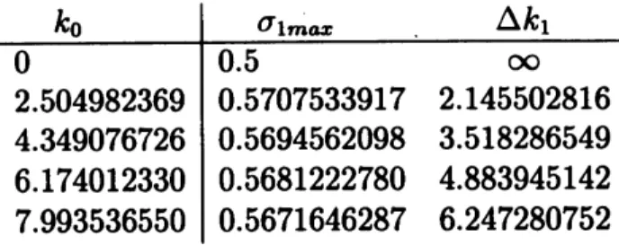
We list in Table 1the numerical values of$\sigma_{1\max}$ and $\Delta k_{1}$ for afirst few intersection points

with $\omega_{0}=0$

.

In the short-wavelength regime $(k\gg 1)$, (4.13) and (4.14) become

$\sigma_{1\max}$ $=$ $\frac{9}{16}(1+\frac{1}{12k_{0}}-\frac{7}{48k_{0}^{2}}+\frac{5}{64k_{0}^{3}}+\cdots)$ , (4.15)

$\Delta k_{1}$ _{$=$ $\frac{3k_{0}}{4}(1+\frac{1}{3k_{0}}+\frac{5}{24k_{0}^{3}}+\cdots)$}

(4.16)

Table 1: The maximum growth rate $\epsilon\sigma_{1\max}$ and the half-wi th $\epsilon\Delta k_{1}$ of unstable band to

$O(\epsilon)$

.

The

case

of$\omega_{0}=0$

The leading term of (4.15) is the well known value of the growth rate for the elliptical

instability elaborated by Waleffe (1990). Roughly speaking, the Moore-Saffman-Tsai-Widnall instability for the static

waves

comprises the long-wave displacement instability and the short-wave instability. The latter is akin to and gives way, in the short-wave

limit, to the elliptical instability.

4.3

The

case

of

$\omega_{0}\neq 0$

The general

case

of$\omega_{0}\neq 0$ is dealt with in parallel with the

case

of$\omega_{0}=0$

.

Likewise,

a

general solution of(4.4) finiteat $r=0$isexpressible solely intermsof the Bessel functions:

$\pi_{1}^{(\pm)}=J_{1}(\eta_{\pm}r)\beta_{1}^{(\pm)}-\{\frac{4\omega_{1}k_{0}^{2}}{(\omega_{0}\mp 1)^{3}\eta\pm}-k_{1}\frac{\eta\pm}{k_{0}}\}rJ_{0}(\eta_{\pm}r)\beta_{0}^{(\pm)}$

$- \{\frac{1}{4}\eta_{\mp}rJ_{0}(\eta_{\mp}r)\mp\frac{(\omega_{0}\mp 1)^{2}(\omega_{0}+3)(\omega_{0}-3)}{32\omega_{0}}J_{1}(\eta_{\mp}r)\}\beta_{0}^{(\mp)}$ , (4.17)

where$\beta_{1}^{(\pm)}$ is constant. Asanticipated at the end of\S 4.1, (4.17)divergeswhen$\omega_{0}=0$

.

In

\S 4.2, this singularity

was

curedby virtually makingthecoefficient$\beta_{1}^{(\pm)}$of the homogeneous

part in (4.17) infinite so

as

to cancel this infinity.

Repeating the

same

procedure,

we

eventually obtain theexpressions of$\sigma_{1\max}$ and $\Delta k_{1}$

.

The detail is reported elsewhere

as

they

are

lengthy. They

are

evaluated numerically at

many of intersectionpoints,showing $|{\rm Im}\omega_{1}|>0$with

no

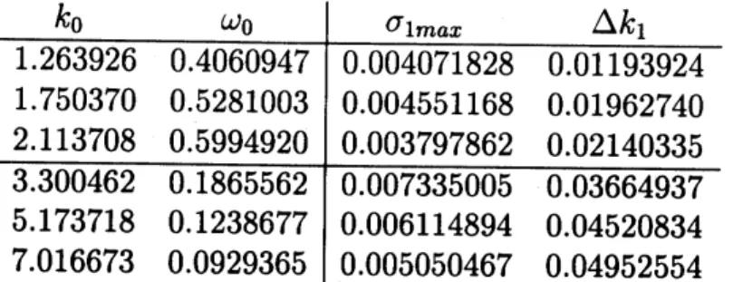
exception. Table 2accommodates

the numerical results for afew crossingpoints that

occur

along the branch of the second

radial mode and offthe axis of$\omega_{0}=0$ but close to it.

Onlythe first

row

$(k_{0}\approx 1.263926)$ agreeswith the numerics of TW76 uptothe firsttwo

digits, butfor theothers,

no

digit ofnumericalvaluescoincideswith the corresponding

one

of TW76. Comparing with Table 1, we confirm the exclusive prevalence of non-rotating modes.

5Energetics

X We are reminded of the point that the spectral stability of aHamiltonian system can

be lostonly by eigenvalue collisions ofpositive- and negative-energy

waves or

by collisions

Table 2: The maximum growth rate $\epsilon\sigma_{1\max}$ and the half-wi th $\epsilon\Delta k_{1}$ of unstable band to

$O(\epsilon)$

.

The

case

of$\omega_{0}\neq 0$

of eigenvalues at 0(Krein 1950; MacKay 1986). Thus

we are

tempted to evaluate the

energy

of the Kelvin

waves.

Cairns (1979) invoked

an

analogy from plasma physics and devised atrick for

calcu-lating

wave

energy that dispenses with adetailed knowledge of the global field. For the

moment, weswitch offthe pureshear, but deal with the whole family of the Kelvin

waves.

A fundamental ingredient is the pressure on both edges of the vortex

core

$r=\eta(\theta, z, t)$

as

given by (3.9). Let the augmented pressure

on

the vortex, through the interface $r=\eta$,

acted by the surrounding fluid be $p_{>}(z, \theta, t)$, and the pressure on the surrounding fluid

acted by the internal fluid be $p_{<}(z, \theta, t)$, and pose the following form:

$p_{>}(\theta,$z,$t)=D_{>}A_{0}^{(m)}e^{:(m\theta+k_{0}z-\omega_{0}t)}$, _{$p_{<}(\theta,$z,}$t)=D_{<}A_{0}^{(m)}e^{\dot{*}(m\theta+k_{\mathrm{O}}z-\omega_{0}t)}$

.

(5.1)

Set the difference of the coefficients

as

$D(k_{0},\omega_{0})=D_{>}(k_{0}, \omega_{0})-D_{<}(k_{0},\omega_{0})$ . (5.2)

The requirement _{of continuity} $D=0$ _ofpressure

across

the interface is no other than the

dispersion _{relation. Cairns’ formula prescribes the wave energy} $E^{(m)}$, per unit length in

$z$, to be

$E^{(m)}=- \frac{\pi}{2}\omega_{0}\frac{\partial D}{\partial\omega_{0}}(A_{0}^{(m)})^{2}$ (5.3)

We recall the pressure $P_{0}$ of the Rankine vortex and the disturbance pressure $\pi_{0}^{(m)}$

inside the

core.

Puttingthese together and using the dispersion relation,

we

can

evaluate

$P_{0}+\pi_{0}^{(m)}\exp[i(m\theta+k_{0}z-\omega_{0}t)]$ _at

$r=\eta-0$ to first order in

wave

amplitude $|A_{0}^{(m)}|$

complying with the form (5.1), with its coefficient provided by

$D_{<}=1- \frac{(\omega_{0}-m)^{2}(\eta_{m}/k_{0})^{2}J_{|m|}(\eta_{m})}{\eta_{m}J_{|m|-1}(\eta_{m})-(|m|+\frac{2m}{\omega_{0}-m})J_{|m|}(\eta_{m})}$

.

(5.4)

The disturbance pressure $\pi_{0}^{(m)}$ in the exterior

region is constructed from the disturbance

velocity potential $\phi_{0}^{(m)}$ through _{$\pi_{0}^{(m)}=i\omega_{0}\phi_{0}^{(m)}-im\phi_{0}^{(m)}/r^{2}$}

.

We evaluate the boundar

value of the augmented pressure at r $=\eta+\mathrm{O}$ as above:

$D_{>}=1- \frac{(\omega_{0}-m)^{2}K_{|m|}}{k_{0}K_{|m|-1}+|m|K_{|m|}}$

.

(5.5)

Difference (5.2) between (5.5) and (5.4) is

$D=(\omega_{0}-m)^{2}\{$$\frac{(\eta_{m}/k_{0})^{2}J_{|m|}(\eta_{m})}{\eta_{m}J_{|m|-1}(\eta_{m})-(|m|+\frac{2m}{\omega_{0}-m})J_{|m|}(\eta_{m})}-\frac{K_{|m|}}{k_{0}K_{|m|-1}+|m|K_{|m|}}\}$

.

(5.6)

Provided that $\omega_{0}\neq m$

as

dictated in $(??)$, the condition $D=0$ indeed restores Kelvin’s

dispersion relation (??). The remaining task is simply to takedifferentiation of (5.6) with

respect to $\omega_{0}$ under the constraint of$D=0$

.

By arepeated

use

of $D=0$,

we

eventually

arrive at arepresentation of the

wave

energy in atidy form:

$E^{(m)}= \frac{2\pi\omega_{0}}{\omega_{0}-m}\{1+\frac{(k_{0}/\eta_{m})^{2}K_{|m|}}{k_{0}K_{|m|-1}+|m|K_{|m|}}[$$\frac{2(\omega_{0}+\sqrt)}{\omega_{0}-}\sqrt$

$+( \frac{m(\omega_{0}+m)}{2}+k_{0}^{2})\frac{K_{|m|}}{k_{0}K_{|m|-1}+|m|K_{|m|}}.]\}(A_{0}^{(m)})^{2}$ (5.7)

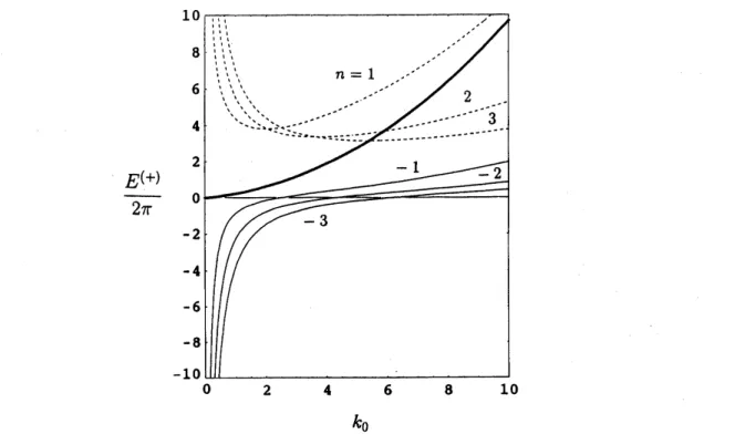
With aview to gaining an insight into the result of\S 4, we sketch in figure 1the wave

energy $E^{(+)}$, divided by $2\pi$, of the left-handed helical

wave

$(m=1)$

as

afunction of

$k_{0}$

.

The

wave

energy of $m=-1$ is exactly the

same

at the

same

value of $k_{0}$ for the

same

order of branch,

as

is evident from the invariance property of (5.7) with respect

to areplacement $m=-m$, $\omega_{0}arrow-\omega_{0}$

.

The

energy

of the primary mode is drawn with

asolid thick line, and that of the first three branches ofretrograde higher radial modes

$(|\omega_{0}|<1)$, counted

as

$n=-1,$_$-2,$-3, and of the first three branches of cograde higher

radial modes $(|\omega_{0}|>1)$, counted

as

$n=1,2,3$,

are

drawn with solid and dashed lines respectively. Here the minus sign is tentatively used in the counter of branch for the sake of convenience. The energy of the primary mode is positive in the entire wavenumber

range. It starts from

zero

at $k_{0}=0$ and increases monotonically with

?.

The energy of

acograde higher mode as well is positive, but it increases without bound

as

$k_{0}arrow 0$ and

monotonically decreases with $k_{0}$

.

The energy of aretrograde higher mode is negative for $k_{0}$ smaller than the value at which the dispersion curve transversally crosses the axis of

$\omega_{0}=0$. It becomes negative infinity in the limit of$k_{0}arrow 0$, monotonically increases with

$k_{0}$, and changes its sign at the intersection point. This singular behaviour is reflective of

confinement of

wave

amplitude in the

core.

The

wave

energy for bending waves, calculated from Cairns’ formula, exhibits

no

con-tradiction with the spectra calculated in

\S 4.

The

resonance

instability of non-rotating

waves $(\omega_{0}=0)$, the dominant one, manifests itselfat adegenerate eigenvalue with

mul-tiplicity two whose eigenfunction has

zero

energy. The

resonance

instability ofrotating

waves

$(\omega_{0}\neq 0)$ stems from

an

eigenvalue collision either between the primary mode and

anegative-energy retrograde higher mode or between apositive-energy and

anegative-energy retrograde higher modes.

$\frac{E^{(+)}}{2\pi}$

$k_{0}$

Figure 1: The

wave

energy $E^{(+)}$, normalized by $2\pi$, of the the bending

wave

with $m=1$

as

functions of $k_{0}$, as given by (5.7). The solid thick line corresponds to the primary

mode, solid lines to the retrograde higher radial modes, and dashed lines to the cograde

higher radial modes.

References

[1] Bayly, B. J. (1986). Phys. Rev. Lett. 57, 2160-2163..

[2] Cairns, R. A. (1979). J. Fluid Mech. 92, 11-14.

[3] Fukumoto, Y.

&Hattori,

Y. (2002). To appear in Proc.

_of

IVTAM Symposium on

Tubes, Sheets and Singularities in Fluid Dynamics (eds. H. K. Moffatt and K. Bajer)

Kluwer.

[4] Krein, M. G. (1950). Dokl. Akad. Nauk. SSSR 73, 445-448.

[5] MacKay, R. S. (1986). In Nonlinear Phenomena and Chaos, Ed. S. Sarkar, Adam

Hilger, Bristol, pp. 254-270.

[6 Moore, D. W.

&Saffman,

P. G. (1975). Proc. Roy. Soc. Lond. A 346, 413-425.

[7] Tsai, C.-Y.

&Widnall,

S. E. (1976). J. Fluid Mech. 73, 721-733.

[8] Waleffe, F. (1990). Phys. Fluids A 2, 776-780.

[9 Widnall, S. E.

&Tsai,

C.-Y. (1977). Phil. Ikans. $Roy$

.

Soc. Lond. A 287, 273-305