Strong Interactions among Particlelike Solutions in Dissipative Systems (Conference on Dynamics of Patterns in Reaction-Diffusion Systems and the Related Topics)

Strong

Interactions

among

Particlelike

Solutions

in

Dissipative

Systems

Research Institute

for

Electronic

Science

Hokkaido University

Yasumasa

Nishiura

Abstract

Three typical transient dynamics in dissipative systems are dis

cussed, namelyself-replication, self-destruction, and scatteringamong

spatially localized patterns. The difficulty lies in the fact that

pat-terns are deformed alot and the associatedorbits behave globally in the phase space. Aconventional treatment in general does not work and needs anew viewpoint to describe them. Our strategy is not to

$\mathrm{t}\mathrm{r}\mathrm{a}\mathrm{c}\mathrm{e}$the orbital behavior iteself, but to search aglobal structure of

networkofbifurcatingsolutionswhichdrives such transient dynamics.

Ahierarchy structureofsaddle-node bifurcationpointsplays acrucial

role for self-replication and self-destruction processes, and unstable patterns called scattors forscattering process. The aimofthis note is to clarify what are the issues and convey the basic ideas to overcome

them.

1Introduction

Scattering ofparticle-like patterns in dissipative systems isstudied, especially

we focus ontheissue how theinput-0utputrelation is controlled at ahead-0n

collisionwhere traveling pulses

or

spots interact strongly. Itremains

an

open

problem due to the large deformation ofpatterns at acolliding point. We

found that special type ofunstable steady

or

time-periodic solutions called

scattors and their stable and unstable manifolds direct the traffic flow of

orbits. Such scattors

are

in general highly unstable

even

in 1D

case

which

causes

avarietyofinput-0utput relationsthroughthescatteringprocess. We

数理解析研究所講究録 1330 巻 2003 年 88-100

illustrate the ubiquity of scattors by using the complex Ginzburg-Landau

equation, the Gray-Scott model and athree-component reaction diffusion

model arising in gas-discharge phenomena.

We focus on the dynamic patterns of spatially localized patterns such

as

pulses and spots in dissipative systems, especially

we are

interested in the

following transient type of dynamics

”_{Self-replication, Self-destruction, and} Scattering”.

The

reason

is thatcomplicateddynamics

as

in Figs 1and 2couldbeobtained

by combination of those dynamics. Fordefiniteness, weemploy thefollowing

Gray-Scott model (see for instance, [2], [15]), although the strategy below

seems to work also for other model systems. Here we only describe the

outline of the results, the readers

are

encouraged to consult the reference

such

as

[10], [11], [12], [13], and [14]. See also the related reference [7], [8],

[9].

$\{$

$\frac{\partial u}{\partial \mathrm{t}}=D_{\mathrm{u}}\Delta u-uv^{2}+F(1-u)$

$\frac{\partial v}{\partial t}=$ $D_{v}\Delta v+uv^{2}-(F+k)v$,

(1)

The simulations depicted in Figs 1and 2show

some

aspectsofthe dynamics

built in this system. The issues

are

1. Self-replication and self-destruction and their relevance to understand

complex spati0-temporal dynamics.

2. Scattering phenomena through collisions among particlelike patterns.

In Fig. 1ordered states

are

observed locally in space and time, however

those

are

transient patterns and the orbits itinerate several different states

through splitting and destruction. Scattering phenomenalike Fig.7 and Fig.8

showpeculiar type of solutions called scattors to which the orbits comeclose

near transitionpointsof input-0utput relations. However from mathematical

point of view there

are

acouple of difficulties to overcome, namely

$\bullet$ The patterns

are

deformed to alarge extent.

$\bullet$ The orbits itinerate globally in the phase space.

$\bullet$ It is not aproiori clear how to reduce the dynamics into finite

dimen-sional space.

Figure 1: $2\mathrm{D}$ SaptiO-temporal chaos for the Gray-Scott model.

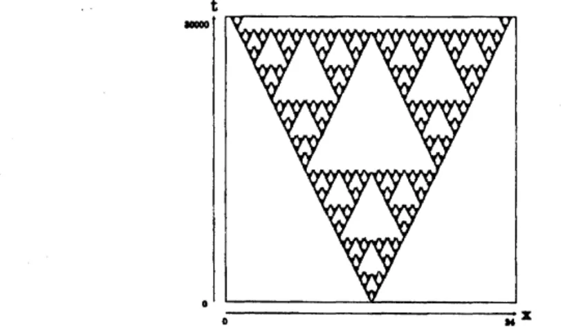
Figure 2: Spatio temporal _self-similar pattern for the Gray-Scott model.

Self-replication and annhilation

are

combined together to create aSierpinski

gasket-like patterns. This

was

first found by Hayase and Ohta [6] for the

reaction-diffusion system of Bonhoeffer-van der Pol type.

It

seems

an appropriate computational approach is indispensable to find

mechanisms which drive those dynamics, and then set up aframework for

rigorous analysis. Conventional techniques such as bifurcation analysis,

sin-gular perturbation, and

some

asymptotic methods areuseful to someextent,

however those are not sufficient to clarify the most essential aspect. It turns

out that aset of bifurcating branches form anetwork in an organized way

and it becomes ahidden mechanism driving the orbits in various ways. This

note is based

on

the joint works with D.Ueyama, K.-I.Ueda, S.-I.Ei and

T.Teramoto.

2Weak and

strong

interactions

among

par-ticlelike

patterns

Atypical example of strong interaction isthe annihilation oftraveling pulses

of the FitzHugh-Nagumo equations at head-0n collision, which still remains

open problem in rigorous

sense.

Self-replication and self-destruction

as

in

Fig.l belong to another category of strong interaction, namely the pattern

splits or destructs by iteself. The following two complimentary approaches

may work well

\bullet Pulse interaction approach with instabilities.

\bullet To find ageometric characterization for the set of global

sx

lution branches which drives such dynamics.

Theformerone is aperturbativemethod and

was

initiatedby physists,

how-ever rigorous analysis is rather recent (see. for instance, [3], [4], [5] ). The

latter one developped by [10], [11], [14]

owes

very much to the recent

devel-opment of fast computer and path-trackingsoftware like AUTO([I]).

3Self-replication

and

self-destruction

Unlike soliton pulses the localized pulses in dissipative systems

can

dupli-cate and annihilate spontaneously. One may think that the dynamics of

self-replication has nothing to do with the destruction process, however it

turnsout that they have basicalythe

same

structure ffombifurcationalview

point, namely they share the

common

structure called “hierarchy structure

of saddle-node points”. See

more

precisely [14]. Here

we

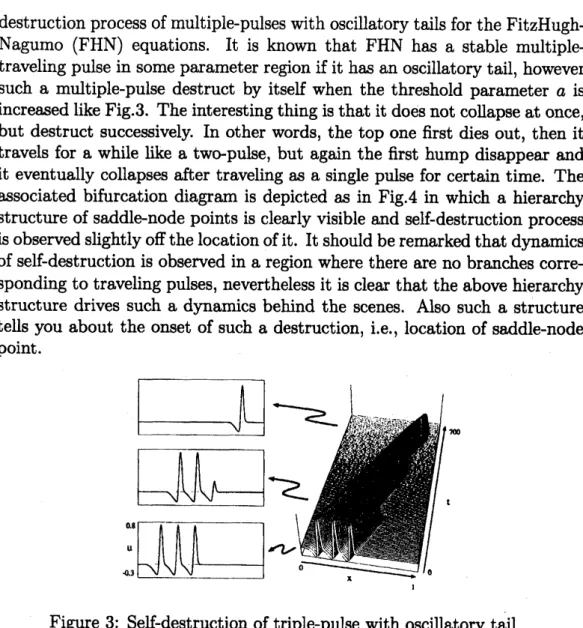
briefly describe the

destruction process ofmultiple-pulseswith oscillatory tailsforthe

FitzHugh-Nagumo (FHN) equations. It is known that FHN has astable

multiple-travelingpulse in someparameter region ifithas an oscillatorytail, however

such amultiple-pulse destruct by itself when the threshold parameter $a$ is

increasedlikeFig.3. Theinteresting thingis that it doesnot collapseat once,

but destruct successively. In other words, the top

one

first dies out, then it

travels for awhile like atw0-pulse, but again the first hump disappear and

it eventually collapses after traveling as asingle pulse for certain time. The

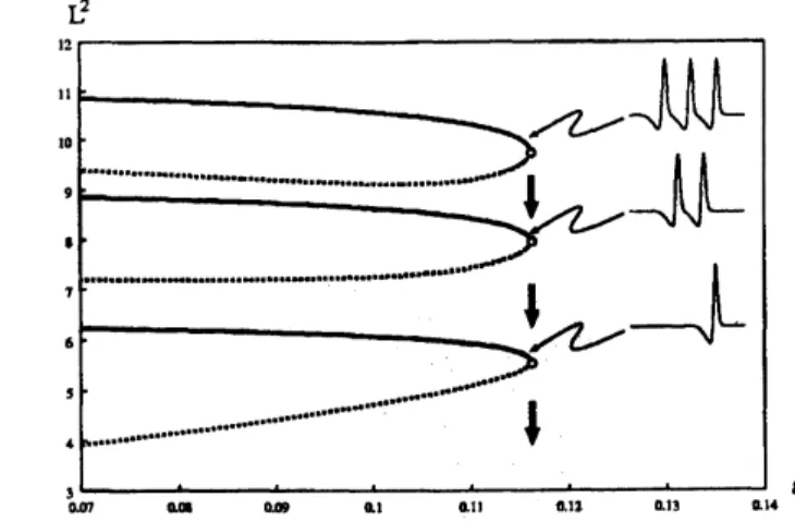
associated bifurcation diagram is depicted

as

in Fig.4 in which ahierarchy

structure of saddle-node points is clearly visible and self-destruction process

isobservedslightlyoff thelocationof it. It should be remarked thatdynamics

ofself-destruction is observed in aregion where there

are no

branches

corre-sponding to traveling pulses, nevertheless it is clear that the above hierarchy

structure drives such adynamics behind the

scenes.

Also such astructure

tells you about the onset of such adestruction, i.e., location of saddle-node

point.

Figure 3: Self-destruction oftriple-pulse with oscillatory tail.

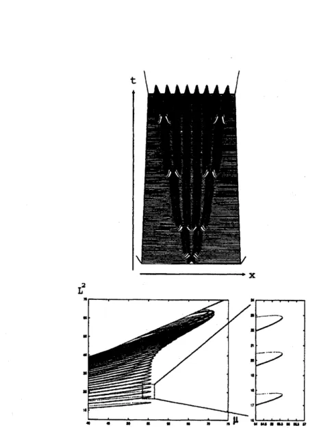
Self-replication is an inverse process of the above destruction dynamics,

namely the unstablemanifold ofsay, one-hump pattern is connected to

tw0-hump pattern, i.e., the increasing direction. Here

we

only show aglobal

bifurcation diagram for the

Gierer-Meinhardt

model arising in the morpho

genesis

as

in Fig.5. It is clearly

seen

that hierarchy structure of saddle-node

points drives self-replication dynamics

as

in the above evolution numerics

of Fig.5 where pulses repel each other and its number increases not like

$arrow 2arrow 4arrow 8$ proportional to $2^{n}$, but $1arrow 2arrow 4arrow 6$

.

This is because only pulses

located at the edge

are

able to split. We

can

prove the edge splitting

phe-nomena

rigorouslyby using pulse-interaction method [4]. The principal part

$\mathrm{L}^{2}$

$\mathrm{a}$

Figure4: Globalbifurcation diagram for multiple-pulseswithoscillatorytails.

The abscissa is the threshold parameter $a$ and the ordinate shows

anorm

of

the pulses. The locationof each saddle-node point coincide almost perfectly

and self-destruction

occurs

when $a$ exceeds this critical point.

of the resulting equations read

$\dot{h}_{1}$

$=-M_{0}(e^{-\alpha h\mathrm{a}}-2e^{-\alpha h_{1}})$

$.\dot{h}_{j}$ $=-M_{0}(e^{-\alpha h_{j-1}}-2e^{-\alpha h_{\mathrm{j}}}+e^{-\alpha h_{j+1}})$ $h_{N}$ $=-M_{0}(e^{-\alpha h_{N-1}}-2e^{-\alpha h_{N}})$

(2)

$\dot{r}_{0}$ $=M_{1}r_{0}^{2}-\epsilon M_{2}-M_{3}e^{-\alpha h_{1}}$

$\dot{r}_{N}\dot{r}_{j}$ $=M_{1}r_{N}-\epsilon M_{2}-M_{3}e^{-\alpha h_{N}}=M_{1}r_{\dot{\S}}^{2}-\epsilon M_{2}-M_{3}(e^{-\alpha h_{\mathrm{j}+1}}+e^{-\alpha h_{\mathrm{j}}})$

where $r_{j}$ denotes the depth of dimple of each pulse, $h_{j}$ the distance between

pulses, $\epsilon$ signed distance from the saddle-node point and all the coefficients

$M_{j}$

are

positive. Note that the equations for $h_{j}$ decouple the equations for

$r_{j}$, therefore it

can

be analysed independently. In fact $h_{j}$ basically increases

monotonically due to the repulsion, onthe otherhand, whether aconcerning

pulse splits or not is determined by whether $r_{j}$ starts to increase rapidly

or

remains finite. In view of the right-hand side of $r_{j}$, the intercept of the

parabola is crucial for this. It turms out that the pulse with the largest

$h_{j}$ primarily starts to split, and such pulses should be located at edge, i.e.,

edge-splitting ([4]), which is consistent with Fig.5.

Figure5: Self-replicationprocessfor theGierer-Meinhardtmodel. Theupper

one

shows the evolution in 1D

case.

The lower

one

is the associated global

bifurcationdiagramforthe set of$\mathrm{N}$-humpstanding pulses

on

afinite interval.

The bifurcation parameter $\mu$ is the decay-rate for the inhibitor.

4

SpatiO-temporal

chaos with

replication

and

destruction

It may be achallenge to construct aexotic transient dynamics, say

spati0-temporal chaos by piecing replication and destruction together. One of the

difficulties is how to tune parameters not to fall in aattractor but to keep

each characteristic dynamics. Recall that the destruction process of

muti-pulses in Fig.3 ends up with the stable rest state and nothing happens after

that. We need to somehow destabilize the final state and activate it to

re-enter into anontrivialstate. This is arealglobal problemandcomputational

approach is indispensabletoclarify the situation. Oneofthegoodcandidates

for mechanisms creating such adynamics is generalized heteroclinic cycle in

infinite dimensional space (see Fig.6). See [11] for details.

5Scattering

among particlelike patterns

So far

we

consider the destabilizations of localized patterns by themselves,

i.e., without interaction with other patterns. The other important class of

strong interactions is scattering among moving localized objects. Avariety

of different types of input-0utput relations are reported in experiments and

numerics (see the reference in [12], [13]). Genericaly in dissipative systems

not only the velocity and the profile ofthe traveling objects but also

input-output relationdepends on the parameters. The detailed process connecting

input tooutput duringthe collisionis quitehardtodescribeevennumerically,

therefore it is necessary to introduce

anew

viewpoint. What

we

present

here is the special type of unstable patterns called scattors which control

the flows

near

the transition points. Originally this

was

strongly motivated

by the numerics on the head-0n collision of 1D pulses for the Gray-Scott

model when the parameters

are

chosen to be close to the transition point

from annihilation to repulsion. The stable manifold of the scattor is loosely

speaking

an

infinite-dimensional version ofseparatrix in ODE, however it is

much

more

subtle and difficult to find it even by numerics. Here

we

only

present just

one

example of such ascattor arsing in the Gray-Scott model.

For

more

details and applications to other model systems,

we

refer to [12]

and [13].

From repulsion to annihilation

First $F$ is fixed to be 0.0198 and study asymmetric coUision. When $k$ is

increased and exceeds $k_{c}\approx 0.0497859$, the input-0utput relation changes

from annihilation (A) to repulsion (B)

as

in Fig.7. The input-0utput relation

depends

on

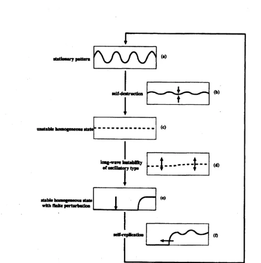
the initial condition, therefore in order to make the transition

Figure 6: Heteroclinic cycle

on

the infinite line passing through aunstable

homogeneous state $P,$ $(1,0)$, and aspatially periodic pattern for the

Gray-Scott model. The homegeneous state $P$ is unstable for large wave-length

region originated from Hopf instability. Strictly speaking, such acycle does

not exist on afiniteinterval, since $(1, 0)$ is stableinthePDE sense. However,

after replacing $(1, 0)$ by $(1, 0)$ with trigger (the resulting cycle is called

a

generalizexl_heterocliniccycle),wecanobserve

an

aftereffect of thegeneralized

cycle numerically. Here, $(1, 0)$ with trigger

means

that there is

some

portion

of the interval where $(u, v)$ is notequal to $(1, 0)$ and from which areplication

wave

can

start propagating.

$\mathrm{u}^{\wedge}j^{\bigwedge_{\mathrm{i}}}$ ’ ’

$0l-\mathrm{F}_{-\mathrm{T}}^{\mathrm{r}\prime^{\prime\approx}}.\ovalbox{\tt\small REJECT}_{-}^{1}.$

’

(B) (C)

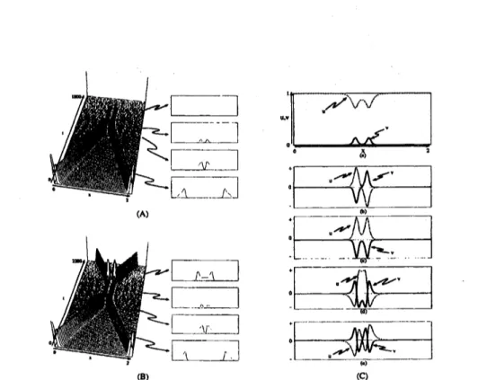
Figure 7: Symmetric collisions for $F=0.0198$

.

(A) Annihilation

occurs

at

$(k, F)=(0.0497859, 0.0198)$

.

(B) As $k$ is slightly increased to 0.0497860,

transition from annihilation to repulsion

occurs.

Note that just before the

occurrence of annihilation or creation of counter-propagating pulses, both

orbits in (A) and (B) stay very close to the separator depicted in (C)(a).

Only$v$-componentis shownin (A) and (B). (C)(a)Theprofileof theunstable

steady state of $\mathrm{c}\mathrm{o}\dim 3$ (scattor). Three unstable eigenfunctions $\phi_{1},$$\phi_{2},$$\phi_{3}$

are

depicted

as

$(\mathrm{b})-(\mathrm{d})$, and (e) corresponds to the Goldstone mode. The

associated eigenvalues

are

$\lambda_{1}=0.06389>\lambda_{2}=0.06378>\lambda_{3}=0.00233$

.

Thefirst two eigenvalues

are

muchlargerthan the first one. Thesolid (gray)

line indicates $v(u)$-component.

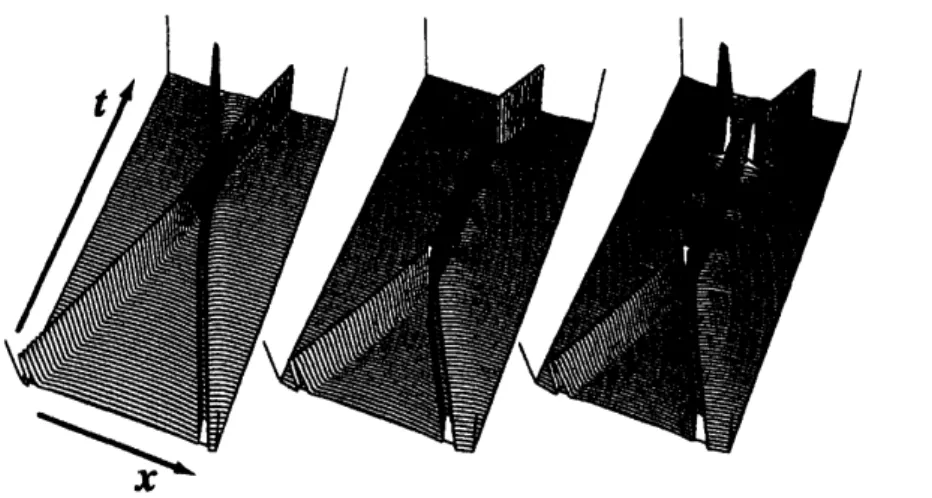
Figure 8: Three different type of input-0utput relations for the

three-component model. Repulsion (left):Tw(\succ into-two case. Number of emitting

pulses

are

preserved. Fusion(middle): Two into

one

case.

After merging, the

fused pattern oscillates for awhile, then emits one traveling pulse. Oscilla

tory repulsion (right): TwO-int0-two case. Two traveling pulses fused into

one

localized wave, then oscillates for certain time, and finnaly splits into

two counter propagating pulses. See [13] for details.

point $k_{c}$ to bewell-defined,

we

have to specify the class of initial conditions.

Theoretically

we

employ asymmetric pair of true traveling pulses

as an

initial condition, which starts initially at $x=\pm\infty$ and collides at the origin.

Practically such

an

initial data and the resulting $k_{c}$

are

well approximated

by takingawell-settled symmetric pair ofpulses. Aremarkable thing is that

there appearsaquasi-steadystate oftwin-horn shape rightaftercollisionand

the orbit approaches it, stays there for certaintime, then annihilate

or

emit

two pulses. In fact thereexists areal steady stateof twin-horn shape, which

is numerically confirmed by the Newton method as in Fig.7. This is what

we call ascattorfor the Gray-Scott model. Alinearized eigenvalue problem;

$L\phi=\lambda\phi$ where $L$ is the linearized operator of the right-hand side of the

system (1) around the twin-horn steady state has three unstable eigenvalues

$\lambda_{1}=0.06389>\lambda_{2}=0.06378>\lambda_{3}=0.00233$ besides the

zero

eigenvalue

A4

coming from thetranslation invariance (see Fig.7(C)). Note that the first

two eigenvalues

are

much larger than the third one, hence the dynamics is

basicaly controlled by$\lambda_{1}$ and $\lambda_{2}$

.

The associated eigenfunctions

are

denoted

by $\phi_{:}(i=1, \cdots, 4)$

.

The twin-horn scattor plays arole as atraffic controller

at collision. Infact,forsymmetrichead-0ncollision,the second eigenfunction

plays

an

important role to determine the fate of the orbit, namely, adding

its small constant-multiple perturbation to the twin-horn pattern, then the

resulting behavior is either annihilation or emissionof two pulses depending

onits signofconstant. Inother words theoutput

can

beclassified by looking

at the response ofthe separator alongthe unstable manifold. In this section

weproposedanewviewpointfrom scattors. Scattors may be unstablesteady

states or time-periodic solutions and their codimensions (i.e., the number

of unstable eigenvalues) is in general high and the origin of adiversity of

input-0utput relations

can

be reducedto the localdynamics around scattors.

We illustrated this viewpoint by using the Gray-Scott model. The orbit

typically approachesascattorrightaftercollisionandissorted outgenerically

along one of the unstable directions ofit. The output

can

be predictable by

using the information on the solution profile right after collision, scattorss

and their unstable eigenforms. Scattorss in dissipative systems

seems

to be

ubiquitous and useful to understand the scattering process, in fact

even

in

higher dimensional space such separators

are

recently found numerically for

various modelsincluding the 3-component system presentedin Fig.8. See[13]

for details and forthcoming articles..

References

[1] E.J.Doedel, A.R.Champneys, T.F.Fairgrieve, Y.A.Kuznetsov,

B.Sandstede and X.Wang,AUTO97..Continuation and

bifurca-tion

_software

_for

ordinary

_differential

equations (with HomCont),

$\mathrm{f}\mathrm{t}\mathrm{p}://\mathrm{f}\mathrm{t}\mathrm{p}.\mathrm{c}\mathrm{s}$.concordia.$\mathrm{c}\mathrm{a}/\mathrm{p}\mathrm{u}\mathrm{b}/\mathrm{d}\mathrm{o}\mathrm{e}\mathrm{d}\mathrm{e}\mathrm{l}/\mathrm{a}\mathrm{u}\mathrm{t}\mathrm{o}$,(1997).

[2] P.Gray and S.K.Scott,Autocatalytic reactions in the isothemlal,

contin-uous stirred tank reactor: oscillations and instabilities in the system $A$

$+\mathit{2}Barrow \mathit{3}B,$ B $arrow C$,Chem. Eng. Sci. Vo1.39(1984) 1087-1097.

[3] Shin-IchiroEi, Masayasu Mimuraand MasaharuNagayama, Pulse-pulse

interactionin

_{reaction-diffusion}

systems, Physica D, $165(2002)176- 198$

.

[4] Shin-Ichiro Ei, Yasumasa Nishiura and Kei-ichi Ueda, $2^{n}$-splitting

or

Edge-splitting -A Manner

_of

splitting in dissipative systems, Japan

J.Ind.Appl.Math. 18(2) (2001)181-205.

[5] Shin-Ichiro Ei, Yasumasa Nishiura and Kei-ichi Ueda, Splitting

_of

trav-eling

waves

in reaction

_diffusion

systems with monO-stable excitability,

preprint.

[6] Y.HayaseandT.Ohta, Sierpinski Gasketin a

_{Reaction-Diffusion}

system,

PRL 81(8)(1998) 1726.

[7] W.N.Reynolds, S.Ponce-Dawson, and J.E.Pearson Self-replicating spots in

_{reaction-diffusion}

systems, Phy.Rev.E 56,

_185-198

(1997).

[8] A.Doelman, W.Eckhaus, and T.Kaper Slowly-modulated twO-pulse

s0-lutions in the Gray-Scott model II..geometric theory,

_bifurcations

and

splitting dynamics SIAM J.Appl.Math. 61, 2036-2062 (2001).

[9] C.Muratov and V.Osipov $\pi aveling$ Spike AutO-Solitons in the

Gray-Scott Model Physica D $155,112- 131$ (2001).

[10] Yasumasa Nishiura and Daishin Ueyama, A

skeleton stretcture

_of

self-replicating dynamics, Physica D, $130(1999)73- 104$

.

[11] Yasumasa Nishiura and Daishin Ueyama, Spati0-tempomlchaos

_for

the

Gray-Scott model, Physica D $150(2001)137- 162$

.

[12] YasumasaNishiura, TakashiTeramotoand Kei-ichi Ueda Scattering and

separators in dissipative systerres, to appear in PRE.

[13] Yasumasa_{Nishiura, Takashi Teramoto and Kei-ichi Ueda Dynamic}

tran-sitions through scattors in dissipative systems, to appear in Chaos.

[14] Yasumasa Nishiura, Far-from-equilibrium Dynamics, AMS, (2002).

[15] J.E.Pearson., Complex patterns in a simple system, Science

$\mathrm{V}\mathrm{o}\mathrm{l}.216(1993),189- 192$

.