Bifurcation analysis of the transition to turbulence in high symmetric flow (Anatomy of Turbulence : Flow Structure and Its Function)

(1)

Bifurcation

analysis

of the transition to turbulence

in

high

symmetric

flow

Lennaert

van

Veen,

Kyoto University, Department of

Mechanical

Engineering

Email:

veen@mech.kyoto-u.ac.jp

March

2,

2004

Abstract

Two scenarios leading to chaos and turbulence in high symmetric flow are de

scribed. Exploiting the symmetries and the divergence free conditionthe number of

degrees of freedom, and thereby the computational effort, is reduced by a factor of

about 300 compared to generaldirect simulation offluid flow. This allows for

bifur-cation analysis at the transition points. At the first transition a sequence of torus

doublings leads to temporalchaos, but the flow doesn’t become turbulent. At lower

viscositythe Ruelle Takens scenarioisfollowedandweareat the onsetof turbulence.

Some differences between these transitions are discussed in the light of bifurcation theory of invariant tori.

1 Introduction

Direct numerical simulation of flows at high Reynolds number requires solving large

sys-temsofdifferentialequations. Forthesolutions toberealistic the smallest resolvedspatial

scale should be ofthe

same

order

as

the typical size of the smallest vortices,

a

fewtimes Kolmogorov’s dissipation scale. As the total number ofdegrees offreedom scales

as

the

cubeofthe ratioof the largest to the smallest resolved scale the limitations ofmemory size and computation time

are soon

met. One way around this problem is to impose spatial symmetries onthe solutions.

In the absence ofboundaries the incompressibleNavier-Stokes equations

axe

invariant

under translations$(\mathbb{R}^{3})$

,

rotations (SO(3)) and reflections$(\mathbb{Z}_{2}^{3})$

.

InKida (1985) a subgroup

ofsymmetries consistingof three finite rotations and three reflections is imposed

on

the

solutions in aperiodic box. Interms of finite truncations in Fourierspace his reduces the

number of independentmodes by

a

factor ofabout 200. The resulting flow displays fully developed turbulencefor low viscosity, whereas only

a

few hundred degrees offreedom

are

necessary to capture spatial scales small enough for reliable simulation. High symmetric

flow

was

subsequently used to explore the statistics of turbulent motion at moderate

Reynolds numbers (Kida

&

Murakami, 1989) and to find evidence for the Ruelle-Takens

(1971) scenario at the transition from regular to chaotic motion Kida et al. (1989). In the latter paper a combination of forward time integration and power spectra

was

used tostudythetransitions. Three-periodic motion

was

shownto

occur as

an

(2)

137

twice. At high viscosity temporalchaos

ensues

but the velocity profile remains simple. At lower viscosity vortices

on

smallscales developandturbulence sets in. Inthis work

we

will take

a

closer look at the bifurcation scenarios leading to chaos and turbulence, focusing

on

the differences between the transitions at high viscosity and low viscosity.

Using bifurcation analysis, Poincare sections and power spectrawe show that at high viscosity

a

sequence oftorusdoubling bifurcations leads to chaos. Beyond this transition

thebehaviour alternates between periodic, quasi periodic and chaotic for small variations of viscosity. Reducing viscosity further

we

find

an

intervalwithstableperiodic motion and then a second transition to chaos. Here, the Ruelle-Takens scenario is followed. Beyond

this transition point the flow starts to look turbulent

as

small scale vortices develop.

The behaviour

near

the transition points is discussed in the light of bifurcation theory of invariant tori

as

presented in Broer et al. (1990).

2 The vorticity equation for high

symmetric

flow

Consider

an

incompressible fluid in

a

periodic box $0<x_{1}$,$x_{2}$,$x_{3}\leq 2\pi.$ In terms of the

Fourier representation of velocity and vorticity,

$\mathrm{v}=\mathrm{i}\sum_{\mathrm{k}}\tilde{\mathrm{v}}(\mathrm{k})\mathrm{e}^{\mathrm{j}\mathrm{k}}$

.,

$\omega$ $= \sum_{\mathrm{k}}\tilde{\omega}(\mathrm{k})\mathrm{e}^{\mathrm{i}\mathrm{k}}$ ” ₍₁₎ we have $3\tilde{\omega}_{1}$.(k)

$=\epsilon_{\dot{l}jk}k_{j}k_{l}$ $v\overline kvl-\nu 7$$2_{\tilde{\omega}_{i}}(\mathrm{k})$ $k_{i}\tilde{u}_{\dot{l}}=0$ $\tilde{\omega}_{\dot{l}}(\mathrm{k})$ _$=$

-\epsilon ijk$k_{j}\tilde{v}*(\mathrm{k})$ (2)

where $\nu$ is the kinematic viscosity and the tilde denotes the Fourier transform. In terms

of the

standard

norm

energy and enstrophy

are

given by

$E= \frac{1}{2}||\mathrm{v}||^{2}$ $Q$ $= \frac{1}{2}||\omega||^{2}$ (3)

respectively.

Now consider the following discrete symmetry operations: Si, reflectionsin theplanes

$\mathrm{Z}$given by$x_{i}=\pi$and$R_{\dot{4}}$, rotations

over

$\pi/2$radiants about the lines$l_{i}$ : _$Cj$ $=\pi/2\mathrm{f}\mathrm{o}\mathrm{r}j\neq i.$

The periodic domain with planes of reflection

axes

of rotation is shown in figure (1).

Supposethe$x$-componentofthe velocityfieldis given in the box $[0, \pi/2]$$\mathrm{x}[0, \pi/2]\mathrm{x}[0,\pi/2]$

.

Applying the symmetry operation $R_{2}\circ R_{3}$ yields the $y$-component and $(R_{2}\circ R_{3})^{-1}$ the $\mathrm{z}$-component in that box. Subsequently $R_{1}$, $R_{1}^{2}$,

$R_{1}^{3}$, $R_{2}^{2}$, $R_{2}^{3}$, $R_{3}^{3}$ and $R_{1}^{2}\circ R_{3}$ yield the

velocity field

on

thebox $[0, \pi]$ $\mathrm{x}[0,\pi]\cross[0,\pi]$ andfinally the reflections $S_{1}$, $S_{2}$, $S_{2}\circ S_{1}$, $S_{3}$, $S_{1}\mathrm{o}S_{3}$, $S_{2}\circ S_{3}$ and $S_{1}\circ S_{2}\circ S_{3}$ fill up the whole periodicdomain. Thus only

one

out of three components in

a

volumefraction $1/4^{3}$ determines the wholeflow, whichreduces the

computational effort by

a

factor 192. The divergence free condition is

more

conveniently handled in Fourier space.

Symmetry operations $S_{}$ and$R_{i}$ introduce linear relations between the Fourier

comp0-nents of vorticity. First of all

we

have

(3)

$1_{3}$

$(0,0,\pi)$ $(0.\pi, )$ $(0.0.2\pi)$ $(0.2\pi.2)$

$—’-’$

’-I–

$(\pi 0,\pi)$ $(2\pi.0.2\pi)$ 1 \prime\prime\prime 1

1 1 $\mathrm{v}_{2}$ 1 1 .$\cdot$. $\cdot$. $\cdot$. $1_{2}$ $-’-_{\mathrm{I}}^{1}--’ \int_{1\prime}’\overline{\mathrm{v}_{3}}^{---}----$ $– \frac{1}{\prime\prime \mathrm{r}\mathrm{I}},$ $-’-[$ : : $1_{1}$ 1 1 $.\cdot.\cdot.\cdot\ldots\ldots\ldots\ldots$ .. $\cdot.\cdot.\cdot$ . $(0.\pi 0)$ $|--\mathrm{I}\llcorner’-\prime \mathrm{I}\prime r--$ \prime\prime – $\mathrm{I}\mathrm{I}$ (0.2.0)

$(\pi,0.0)$ $(\pi$

.

.0$)$ $(2\pi,0,0)$ $(2\prime 2\pi,0)$

Figure 1: Left: the domain $[0, \pi]$ $\mathrm{x}[0,\pi]\mathrm{x}[0, \pi]$ with theaxes ofrotation $l_{1,2}$,s drawn in. Right:

the domain $[0, 2\pi]$ $\mathrm{x}[0,2\pi]\mathrm{x}[0,2\pi]$with the planesof reflection $V_{1,2,3}$drawnin. If

one

component

of the vorticityfieldisspecifiedin the boxdelimited by thedottedline, thefullfieldontheperiodic

domain follows from symmetry.

so

that

we

may consider only

one

component. This scalar function is

even

or

odd in its

arguments:

$\tilde{\omega}1(k_{1}, k_{2}, k_{3})=\tilde{\omega}1(-k_{1}, k_{2}, \mathrm{c}_{3})=-\tilde{\omega})(k_{1}, -k_{2}, k_{3})=-\tilde{\omega}1(k_{1}, k_{2}, -k_{3})$ (5) and finally

we

have

$\tilde{\omega}_{1}(k_{1}, k_{2}, k_{3})=\{$

$-\tilde{\omega}_{1}(k_{1}, k_{3}, k_{2})$ for $k_{1}$ and $k_{2}$ and$k_{3}$ even,

$\tilde{\omega}_{1}(k_{1}, k_{3}, k_{2})$ for $k_{1}$ and $k_{2}$ and $k_{3}$ odd,

0otherwise.

(6)

We consider

a

cubic truncation, i.e. $|k1,2,3|\leq N.$ Relations $(4)-(6)$ reduce the number of

independent Fourier modesofvorticity by

a

factor of

192

in the leading order, that is $N^{3}$

.

There is, however

one more

linear relation which allows for further reduction, namely the divergence free condition for vorticity. With the aidofrelation (4) it reads

$k_{1}\tilde{\omega}_{1}(k_{1}, k_{2}, k_{3})+k_{2}\tilde{\omega}_{1}(k_{2}, k_{3}, k_{1})+k_{3}\tilde{\omega}_{1}(k3, k_{1}, k_{2})=0$ (7)

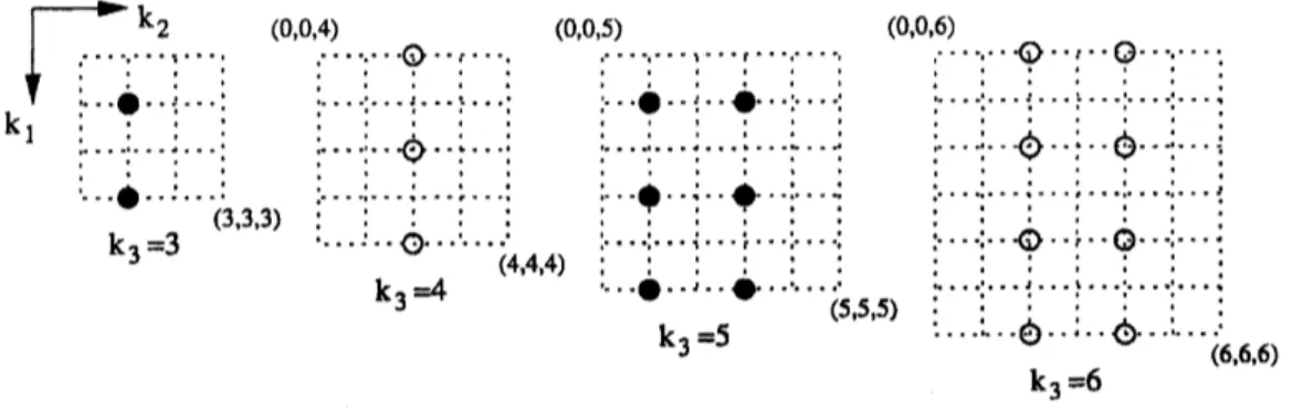
Taking maximal advantage of relations $(4)-(7)$ weconsider only Fourier components of$\omega_{1}$

in the fundamental domain $\{\mathrm{k}\in l^{3}|k_{3}>k_{2}, k_{3}\geq k_{1}, k_{1}\geq 0, k_{2}>0, k_{3}\leq N\}$

.

A sketch

of this domain is shown in figure (2). The number ofindependent modes is reduced by

a

factor of288 in the leading order. These components satisfy the following equation

$\frac{\mathrm{d}}{\mathrm{d}t}\tilde{\omega}_{1}(k_{1}, k_{2}, k_{3})=k_{2}k_{3}(\tilde{S}(k_{3}, k_{1}, k_{2})-\tilde{S}(k_{2}, k_{3}, k_{1}))+k_{1}k_{2}\tilde{T}(k_{2}, k_{3}, \mathrm{c}_{1})$

$-k_{3}k_{1}\tilde{T}(k_{3}, k_{1}, k_{2})+(k_{2}^{2}-k_{3}^{2})\tilde{T}(k_{1}, k_{2}, k_{3})$ $-\nu k^{2}c\tilde{\omega}_{1}(k_{1}, k_{2}, k_{3})$ (8)

where $\tilde{S}$

and $\tilde{T}$

are

theFourier transforms of

(4)

138

$\ulcorner_{1}^{\mathrm{k}_{2}}|\mathrm{i}.\cdot.\cdot..\cdot\cdot.\cdot\cdot.\cdots\backslash |\dot{\mathrm{o}}\cdot\cdot i|.\cdot\cdot\cdot.\cdot...\cdot..\cdot$

. $(0,0,.\cdot..\cdot 4.)|..\cdot\cdot.\cdot.\mathrm{i}_{0}.\cdot..\cdot.\cdot i.\cdot$

..

$\cdot$.-.

..

$\cdot$ $(0,0_{\mathrm{I},1’},.5..)|..\cdot.\cdot|.\cdots.,|.\cdots\cdot..\cdot.\cdot.1||\dot{\mathrm{o}}\cdot\cdot\dot{}\cdot\cdot\dot{\mathrm{o}}\ell\cdot\cdot..\cdot\cdot.\cdot.\cdot.\cdot.||’.||.\cdot$

.

$(0,0_{1},...6..)\mathrm{I},.\cdot\cdot.\cdot.\cdot..\cdot$

..

$\cdot.\cdot\cdot.\mathrm{Q}.\cdot.\cdot\cdot\cdot\cdot\cdot\ldots|\cdots||...\cdot$. $\cdot$ $...\cdot...\cdot.\cdot..\cdot\cdot.\backslash \cdot.\cdot$. $\mathrm{k}1$ $||\ldots$.$\cdot\ldots\ldots$.: $.\cdot..\cdots.\mathrm{I}.\cdot..\dot{.\cdot}...\cdot$

.

$\cdots\cdot.\cdot$

.

$|.\cdot\ldots.||.\cdot.\cdots...\cdots\cdot.\cdot\ldots..\cdot.\ldots..\cdot.\cdot$ $.\cdot.\cdot\ldots..\cdot.\cdot.$.

(...

$\cdot$$\cdot$

;

$\cdot\cdot \mathrm{O}^{\iota}\cdots.\cdot..\cdot\ldots i.$

.

$|.\cdot\ldots \mathrm{k}_{3}.=.3i.\cdot.\cdot$

...$(.\cdot.3,3,3)$

$.\cdot.\cdot...\cdot.\cdot.\cdot.|||.\cdot..\cdot.\cdot\dot{}’.\cdot.\cdot.\cdot.\cdot.i..\cdot.\cdot.\cdot.\cdot..\cdot$

.

$|\cdots 0\cdot$.$|\cdot\cdot 2$..$..\cdot.\cdot\ldots..\cdot.\cdot$

$.\cdot.\cdot.\cdot..\cdot.\cdot.\cdot.\cdot.\cdot.\cdot..\cdot.\cdot.\cdot.\dot{\oplus^{\backslash }}.\cdot\cdot..\cdot|\cdot..\cdot\cdot||\dot{\mathrm{Q}}|..\cdot.\cdot.\cdot.\cdot||.\cdot\cdot\cdot.\cdot.\cdot.\cdot’.\cdot\cdot$

..

:....:$\ldots$$\{$$\cdots j\cdots.\cdot\ldots.:1$

$\mathrm{k}_{3}4$ (4,4,4) $|\mathrm{i}$ ..$.!^{\iota}$. . $i|$ . .$\dot{\mathrm{o}}$

..

..$\cdot$

.

$\cdot$ . . . .$\cdot$

.

$\cdot$ $.\cdot.\cdot\ldots..\cdot.\cdot\ldots \mathrm{j}\ldots|‘$

.

$\ldots|i||..\cdot.\ldots.|.\cdot.\cdot\ldots...\cdot$

.

(5,5,5) _:

$\mathrm{k}_{3}=5$ $\ldots$.1$..\cdot\cdot|\ldots 6\ldots$$.|.\ldots(.\cdot 6,6,6)$

$\mathrm{k}_{3}=6$

Figure 2: Wave vectors corresponding toindependent amplitudes$\tilde{\omega}_{1}(\mathrm{k})$

.

Shown arethe firstfour

levelsin $k_{3}$, starting at the smallestwavevector$\mathrm{k}=(1,1,3)$

.

Solid: odd sub lattice. Open: even

sub lattice. and

$k^{2}\tilde{v}_{1}=k_{2}\tilde{\omega}_{1}(k_{3}, k_{1}, k_{2})-k_{3}\tilde{\omega}_{1}(k_{2}, k_{3}, k_{1})$ (10)

Energy in supplied by fixingthe low order odd mode $\tilde{\omega}1(1,1,3)=-3/8$

.

Thus

we

obtain

a

family ofdynamical systems with

one

parameter, $\nu$, and

a

number of degrees offfeedom

given by $n(N)=\{)$ $\frac{2}{\frac{32}{3}}(+(\frac{\frac 2N)^{3}N-1}{2})^{3}\frac{1}{+2}(\frac{N}{2(})\frac{7}{\%}\frac{N}{2-}\frac{3}{2}\frac{N-12-}{2})\frac{1}{6}(\frac{N-1}{2})$ if$N$ is odd if$N$ is

even

(11)

3 Numerical considerations

Inperformingtime integrations

we

avoid the

use

of thepseudo spectral methodcommonly employed forthreedimensional simulations. Dueto thereduction ofthe number of degrees

of freedom the direct method is not much slower and yields

a

simple, transparent code

and easy

access

to the Jacobian for integration of the linearised system. The code is composedof twoparts. First, all nonlinear interactioncoefficients

are

computed for

a

given

truncation level $N$

.

This is done by looping

over

all resonant triads for

a

given Fourier

component and mapping all resonant modes onto thefundamental domainby symmetries $(4)-(6)$ and relation (7). This process takes up to a few minutes for truncation levels up

to $N=21,$ the highest resolution considered in Kida et al. (1989). After that

a

seventh

to eighth order Runge-Kutta-Felbergh scheme with step size adjustment is employed for integration. The

use

of

a

high order method might

seem

odd for such large systems but

as

it turns out that the step size adjustment

more

than makes up for the larger number

of

evaluations of the vector field,

13

compared to

4

for

fourth-0rder

Runge-Kutta.

The following experiment

was

done to check this. If

we

do not fix $\overline{\omega}1$(1, 1, 3) in time

and set $\nu=0$ kinetic energy $E$ is conserved. The fourth-0rder and high order Runge

Kutta method

were

employed to integrate the conservative system

over

an

interval $\Delta t$

muchlarger than the typical time scale offactuations, whichis$\mathrm{O}(1)$

.

The

error

tolerance

for the energy conservation

was

fixed to $\kappa\sim$

.

For the high order method this is done by

specifying the local

error

tolerance, for $\mathrm{t}\mathrm{h}.arrow\underline{!}\gamma \mathrm{w}$ ordermethod by choosing asmall enough

(5)

$0\mathfrak{l}$ 01 $\mathrm{V}-$ .00836 $\mathrm{v}=0.0$ 153 01 $00$’ 0 ’ $\mathrm{Q}\eta 0$ , 0 ’

.

’

.

1 0 0 0 0 0 ’ 1 ’ 0 0 0 0 $0S$ 1 kn kn

Figure 3: Band-averaged enstrophy spectra near the transitions to chaos (see section (4)). Ob

tainedfrom anintegrationof$10^{3}$ timeunits, $\log$-linear scaleinnormalised units. Left: atthefirst

transition, $\mathrm{I}\mathrm{I}arrow \mathrm{I}\mathrm{I}\mathrm{I}$ infigure (4). Right: at the second transition,$\mathrm{V}arrow \mathrm{V}\mathrm{I}$

.

the average step size of the high order method is about ten times the required step size

of the low order method. As many ofthe results presented here

are

based

on

rather long time integrations it importantto keep the

error

tolerancelow. The seventhtoeighthorder

long -Kutta-Felbergh scheme has been shown to be extremely reliable,

see

for instance

Tuwankotta

&

Quispel (2003), where this scheme is shown to be

as

accurate as, albeit

slower than, problem-specific symplectic methodsin a nearly integrableproblem.

Below simulations

are

performed with

a

viscosity in the

range

$0.004<\nu<0.01$ and thetruncation level fixed to $N=15.$ We computed theenergyand the enstrophy,

as

well

as

Taylor’s micr0-scale Reynolds number, $R_{\lambda}$

,

and Kolmogorov’s dissipation length scale, $\eta$, defined by

$R_{\lambda}= \sqrt{\frac{10}{3}}\frac{E}{\nu\sqrt{Q}}$ $\eta=\sqrt[4]{\frac{\nu^{2}}{2Q}}$ (12)

As

a

rule of thumb the ratio $\eta||k||_{\max}$ has to be $0(1)$ for the truncation

error

to be

negligible. In the viscosity rangeexploredhereit variesintherange$1.3>\eta||k||_{\max}>$

0.63.

Tomake

sure

the truncation level is high enough to describethe transitions to chaos, the focus of this research,wecomputedthe band-averaged enstrophy spectra at the transition

points, they

are

shown in figure (3). At thesmall scales

an

exponential decay is visible,

indicating that

our

numerical results

are

reliable. Thetime average micr0-scale Reynolds number varies from $R_{\lambda}\approx 55$to $R_{\lambda}\approx 27,$ indicating that onthe lower end of the viscosity

scale

we are

at theonset of turbulence.

In addition to time integration

we

appliednumerical

bifurcation

analysis to thissystem.

For thisend

we

use

the software package

AUTO

(Doedel et$\mathrm{o}\mathrm{Z}.$, 1986). This software is not

designed to handlelarge systems and

a

scaling needs to be introduced for computation of

(6)

141

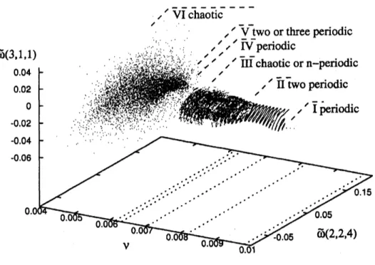
Figure 4: Limit point diagram intherange$0.01>\nu>$ 0.004. Visibleisthetransition$\mathrm{I}arrow \mathrm{I}\mathrm{I}$ from

periodic to quasi periodic, $\mathrm{I}\mathrm{I}arrow \mathrm{I}\mathrm{I}\mathrm{I}$ to chaotic, $\mathrm{I}\mathrm{I}\mathrm{I}arrow \mathrm{I}\mathrm{V}$back to periodic, $\mathrm{I}\mathrm{V}arrow \mathrm{V}$ to quasiperiodic

and $\mathrm{V}arrow \mathrm{V}\mathrm{I}$ to $\mathrm{c}\mathrm{h}\mathrm{a}\mathrm{o}\mathrm{t}\mathrm{i}\mathrm{c}/\mathrm{t}\mathrm{u}\mathrm{r}\mathrm{b}\mathrm{u}\mathrm{l}\mathrm{e}\mathrm{n}\mathrm{t}$

.

In region $\mathrm{m}$the behaviour alternates between chaotic and two

or

threeperiodicwhile the spatialstructure of the flow remainssimple.

4 Transitions to

chaos and

turbulence

The focus of the present paper is the transition from regular to chaotic and turbulent behaviour for decreasing viscosity. In Kida et al. (1989) two and three periodic motion

was

found which implies that the Ruelle-Takens scenario is followed. It

was

also shown that, after

an

initial transition to temporal chaos regular (periodic) motion sets in. $\mathrm{A}\mathrm{f}rightarrow$

ter

a

second transition the spatial behaviour becomes

more

complicated and turbulence

develops. That work

was

mainly based

on

forward time integration, power spectra and

measurement of the micro scale Reynolds number. In addition to these instruments

we

employ bifurcation analysis to take

a

closer look at the transitions.

For large viscosity

an

equilibriumstate is the global attractor for this system. At /83

0.0113 a

Hopf bifurcation

occurs

inwhich

a

stableperiodic orbit is created. To get

a

first

impressionof thetransitions from periodicity to chaoticandturbulent motionwecomputed

a

limit point diagramintherange$0.01>\nu>$

0.004

ofthePoincare map

on

the plane given

by$\tilde{\omega}(0,2,4)=$ 0.005. Theintegration time

was

$\Delta t=1000$ for each parameter value, after

a

transient time of 100 time units, using the last point at the previous viscosity

as

initial

value. The limit pointdiagram isshown in figure(4). Two parameter ranges with periodic

behaviour

can

be

seen: one

for $\nu>$ 0.0105 and

one

around $\nu=$ 0.0068. A continuation

(7)

$\mathrm{z}_{2\mathrm{a}\mathrm{s}_{\mathrm{r}50\mathrm{o}\mathrm{e}\alpha}}\Leftrightarrow.\ovalbox{\tt\small REJECT}_{0\mathrm{o}\mathrm{e}\mathrm{o}0\mathfrak{g}}\mathrm{a}_{\mathit{1}^{1}}235\mathit{3}^{\cdot}$.

$|||\mathrm{I}||1|$

2

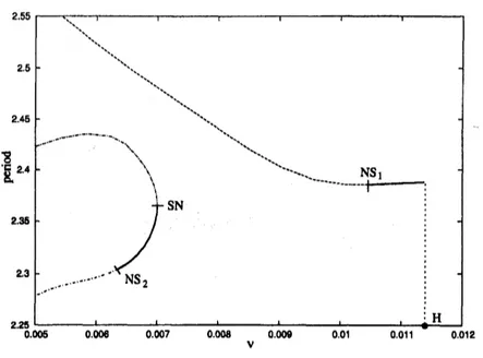
Figure 5: Continuationof two branches ofperiodic solutions,

one

created in Hopfbifurcation$\mathrm{H}$

andonenot connected to abranch ofequilibria. Periodversusviscosity. Thicklines denote stable

orbits, thinlines unstableorbits. SNdenotes asaddle node bifurcation andNS aNeimark-Sacker

(torus) bifurcation.

around$\nu=$

0.0068

doesnotbifurcatefrom

an

equilibrium. Bothbranches become unstable

in

a

Neimark-Sacker,

or

Torus bifurcation. Directly beyond these

bifurcation

points

we

expect the behaviour to be quasi periodic, and indeed invariant circles

appear

in the

Poincare section, figure (4). The transitions which

occur near

bifurcation points NSi and

$\mathrm{N}\mathrm{S}_{2}$

are

different andlead to different behaviour. Inthe following sections

we

willdescribe

the breakdown of the invariant tori in

more

detail.

4.1 The

first

transition to chaos: torus

doubling

bifurcations

As can be

seen

in figure (4) quasi periodicmotion persists

over a

large parameter range to

theleft of bifurcation point$\mathrm{N}\mathrm{S}_{1}$

.

Theoretically

we can

expectthe quasi periodicbehaviour

to persist

on a

ffactal domain in parameter space,

as

proven in Broer et al. (1990)(part

$\mathrm{I})$

.

Therefore we might

see

many transitions. Indeed, to the left of $\mathrm{N}\mathrm{S}_{1}$ we find periodic

(phase-locked) motion, $3arrow \mathrm{p}\mathrm{e}\mathrm{r}\mathrm{i}\mathrm{o}\mathrm{d}\mathrm{i}\mathrm{c}$ motion (as reported

on

inKida et al. (1989)) and chaos.

Transitions betweenthese regimes

can

berelated to bifurcations ofphaselocked orbits,

as

shown in Broer et al. (1998),

or

rather to bifurcations of the torus itself. In Broer et al.

(1990) (part $\mathrm{I}\mathrm{I}$

)

a

partialtheoryof bifurcating toriisdeveloped. In particular quasiperiodic

saddle-node, period doubling and Hopfbifurcations

are

shown to

occur

generically if

one

parameter is varied. The quasi periodic Hopf bifurcation corresponds to

a

transition to

3-periodicmotion, whereas the quasi periodicperiodicdoubling (ortorusdoubling) results either in two new, disjunct tori

or

in

one

new

torus with

one

period doubled. The latter

bifurcation shows up in

our

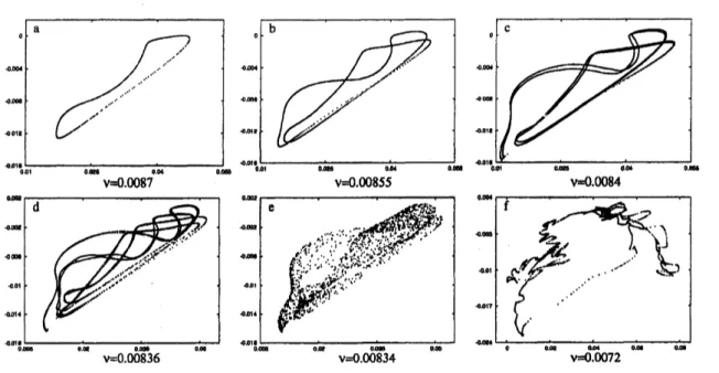
system.

The first transition ffom quasi periodic to chaotic is shown in figure (6). The torus doubles at least three times before

a

chaotic attractor shows up. Cascades of torus

(8)

dou-143

$\infty 4M4M$

*D

$\nearrow’,\nearrow’\mathrm{r}’,\alpha$

$\varpi$

$\triangleleft \mathrm{n}\mathrm{a}\triangleleft m\mathrm{r}_{\rho}M\ovalbox{\tt\small REJECT} \mathrm{m}$’

$J’r^{\nearrow’}u$

$\mathrm{r}$

$\tau \mathrm{r}\triangleleft \mathrm{r}*\ovalbox{\tt\small REJECT}_{\mathrm{o}\mathrm{r}}^{l}\alpha \mathrm{r}_{0\mathcal{M}\mathrm{R}U}4M\mathit{0}$

400 -000 400

$\mathrm{R}$

$\omega \mathrm{r}_{4}\alpha \mathrm{m}\mathrm{c}\mathrm{r}\mathrm{n}\mathrm{r}\prime \mathrm{e}_{\delta}\not\in^{p}\xi_{\beta_{\mathrm{g}^{\vee}}^{\vee}}^{_{}}.\backslash \cdot\prime^{\acute{\{}_{}\prime}.\cdot\dot{j}_{*}..\cdot.\cdot..\cdot.\cdot,\cdot.\dot{t}’_{\mathrm{B}}..’$

.

$\wedge,\cdot.t_{\acute{k}^{*\cdot\acute{}},’}^{j_{\backslash }^{_{\grave{\acute{|}j}’i}}}\dot{.}_{_{l^{\backslash },.\backslash .,},j\cdot,i\dot{j}^{\acute{\mathrm{v}}_{}}}..\cdot..\cdot\cdot..\cdot._{\mathit{3}}..\cdot..\cdot..\cdot...\cdot..i‘.\cdot..\cdot\cdot\sim’.f_{i\cdot!}\acute{\dot{\nu_{\mathrm{s}_{\sim}\mathrm{b}}^{\backslash .\mathrm{e}_{\vee}}|}}\cdot,.\cdot..\cdot\dot{.}’...\cdot.f_{i_{\mathrm{Y}_{\backslash }}^{4}}.’\cdot,i_{\dot{\mathrm{r}}}.\cdot..\cdot_{*}...\ovalbox{\tt\small REJECT}^{\sim.\dot{\Psi}}..\cdot\acute{..1\cdot.}’\oint_{}..|.i.\grave{P}^{\mathrm{t}}$

.

$\triangleleft\rho\prime 0^{\cdot}M$

$0\alpha$

$\mathrm{v}=0.0^{\mathrm{o}\mathrm{m}}0834$

$\mathit{0}oe$

Figure 6: Poincare sections near bifurcation point $\mathrm{N}\mathrm{S}\mathrm{i}$. Integration time for each picture was

$\mathrm{O}(10^{3})$

.

Prom a to $\mathrm{d}$ the invariant torus doubles three times whereas the motion remains quasi

periodic. At $\nu=$0.00834, picture$\mathrm{e}$,the motion hasbecome chaotic. Reducing theviscosityfurther

the torus reappears. In picture $\mathrm{f}$it seems to be near breakdown.

$\mathrm{C}*\ovalbox{\tt\small REJECT}_{0\mathrm{J}}^{0)}\ovalbox{\tt\small REJECT}^{\omega_{2}}\ovalbox{\tt\small REJECT}\ovalbox{\tt\small REJECT}_{\delta 01}^{\omega}\epsilon_{06}\epsilon\epsilon- \mathrm{a}48\mathrm{e}\alpha_{\mathrm{k}}-054\ovalbox{\tt\small REJECT}\ovalbox{\tt\small REJECT}\mathrm{I})2$ $\tau_{\mathrm{P}}\triangleright \mathrm{e}03\triangleright\alpha 09\triangleright\triangleright oe\triangleright_{s\mathrm{a}}\epsilon-3\mathrm{o}\mathrm{e}\ovalbox{\tt\small REJECT}_{3}^{\omega_{2}}\ovalbox{\tt\small REJECT}\ovalbox{\tt\small REJECT}^{01}0)\mathit{0}1_{\mathrm{C}0}$

$0\mathrm{s}$ $25\mathrm{c}\mathrm{r}$

Figure 7: Energy spectrum obtained from an integration with $\nu=$ 0.00834 and $\Delta t=4\cdot$ $10^{3}$

.

Onthe left: low frequency domain withfundamental ffequency $\omega_{2}$ and harmonics

$\omega_{2}/2^{k}$

.

On the

right: highfrequency domainwith fundamental frequency$\omega_{1}$ andsomecombination peaks.

blings

were

reported

on

long before the normal form theory

was

developed, e.g. Kaneko

(1983); Franceschini (1983); Anishenko (1990). In spite of attempts to develop scaling

and normal form theory,

as

in Kaneko (1984); Arneodo et al. (1983), those studies

were

mainly phenomenological and led to the conjecture that, in contrast to doublingcascades

of periodic orbits, only a finite number of torus doubling

can occur

before the torus is destroyed and chaos

ensues.

(9)

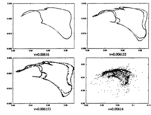
Figure

8:

Poincare sections near bifurcation point $\mathrm{N}\mathrm{S}_{2}$

.

Integration time for each picture was

$\mathrm{O}(10^{3})$

.

Fromato$\mathrm{b}$we seetheinvariantcircledouble

once

but in

$\mathrm{c}$athirdfundamentalffequency

has appeared in a quasi periodic Hopf bifurcation. In picture $\mathrm{d}$ the three periodic motion has

broken down and chaos isobserved. Note, that the scales have been adjusted.

value $\nu=$0.00836, corresponding to Poincar\’e section $(6\mathrm{d})$

.

Frequency $\omega_{1}$ lies close to the

period of the orbit that is stable for $\nu>$

0.0105.

In the low frequency range the other

fundamental frequency, $\omega_{2}$ is shown. The peaks at $\omega_{2}/2^{k}$ for $k=1,2,3$

are

due to the

repeated period doubling. These harmonics also show up in combination peaks,

as

shown

around $\omega_{1}$

.

4.2 The

second transition to

chaos: quasi periodic

Hopf

bifurcation

Stable

quasi periodic motion is again found beyond bifurcationpoint $\mathrm{N}\mathrm{S}_{2}$ (see figure (5)).

The corresponding invariant circle of the Poincare map is shown in figure (8a). If we

decrease the viscosity we first observe

a

torus doubling

as

described above. The double invariant circle isshown in figure (8b). However, subsequent doublingbifurcations

are

not

found. Insteadfor slightlylower viscosity

we

findthree periodic motion. A quasi periodic Hopf bifurcation has occurred and

a

third fundamental ffequency has been created. The three dimensional torus shows up in the Poincar\’e section

as a

thick invariant circle,

see

figure $(8)\mathrm{c}$

.

Aswasshown byRuelle

&

Takens (1971) the threeperiodicmotion is unstable

to perturbations and if

we

decrease viscosity further

a

chaotic attractor shows up $(8\mathrm{d})$

.

Thus, the second transition to chaos follows

a

scenario different from the first

one.

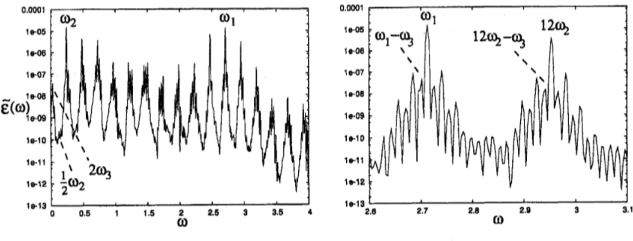
The energy spectrum for three periodic motion is shown in figure (9). The first

fun-damental frequency, $\omega_{1}$, is again related to the period ofthe orbit from which the torus

(10)

145

0 01 2 1 1 05 1 0 ’ 07 0 1 1 ₁₂ ’ 5 1- 12 1 06

$\backslash \backslash \backslash$

$\backslash \backslash \backslash \backslash$ $1$ $7$ $\tilde{\epsilon}()11$ $-$ $\backslash \backslash$ ,-08 .09 1 $-\prime 0$ $\backslash$ 110 $\backslash$ $\backslash$ e-1I $\mathfrak{j}\mathrm{t}\mathrm{t}$ 1 $2 $\frac{1}{2}\backslash 22$ ’ $\dagger 2$

1130

0. 1 15 2 .5 .5 4 ’

12

2.7 $B$ 2.9 3 31

Figure 9: Energy spectrum obtained ffom an integration with $\nu=$ 0.00834 and $\Delta t=4\cdot$ $10^{3}$

.

O$\mathrm{n}$theleft: low frequency domain with fundamental frequency$\omega_{2}$ and harmonics

$i_{2/2^{k}}$

.

On the

right: high frequency domainwith fundamental frequency$\omega_{1}$ and somecombination peaks.

weak, at $\omega_{2}/2$ due to the doubling bifurcation. The third fundamental frequency, $\omega 3$

,

is

fairly small but

we can see

its harmonics.

On

theright hand side

an

enlargement around

$\omega_{1}$ is shown. The system is

near

1 :11

resonance

so

that thepeaksat

$11\omega_{2}$ and$\omega_{1}$ almost

coincide. Combination peakswith the third fundamental frequency

are

shown around $\omega_{1}$

and $12\omega_{2}$

.

5 Conclusion

Takingfull advantage of the symmetries anddivergence ffeecondition we have simulated

high symmetric flow at micro scale Reynolds numbers in the range $R_{\lambda}\approx 27-55$

.

As

reported in Kida et al. (1989),

we see

intervals with stable periodic motion in this range,

followed by

a

transitionto quasi periodicand, subsequently, chaotic motion fordecreasing

viscosity. By the

use

of bifurcation analysis, Poincaresections andpowerspectra

we

have

shownthatthese transitions

are

different in nature. Thefirst transition to chaos is due to

a sequence

of torusdoublingbifurcations. The theory ofsuchcascades is

as

yet incomplete

and scaling laws similar to those for doubling cascades of periodic orbits haven not been

derived. The impression ffom numerical

simulations

andexperiments is that only

a

finite

number of torus doublings

can occur

before chaos

ensues

(Arn\’eodo etal., 1983; Anishenko,

1990). In

our

system

we

observe three doublings, but further integrations might reveal

more

doubling bifurcations, which would contributeto the formulation ofscaling laws. If

we

decrease viscosity beyond the first transition point

we

find

an

interval in

pa-rameter space with many transition between periodic, quasi periodic and chaotic motion. This is in agreement with the theory formulated by Broer et al. (1990), which says that quasi periodic motion will be stableon afractal set in parameterspace. Inthis region the spatial structure of the flow remains simple andonly large scale vortices arise.

Thesecond transitionis shown to follow the

Ruelle-Taken

(1971) scenario, periodic $arrow$_?

tw0-periodic $arrow$threeperiodic$arrow$?chaotic. Poincar\’esections showthat

a

chaoticattractor is

(11)

process. This attractor persistsfordecreasing viscosityasthe microscale Reynolds number exceeds 50 and turbulent motion sets in.

The difference in behaviour beyond the transition points through quasi periodic

dou-bling and quasi periodic Hopfbifurcationsleads tothe hypothesis thatquasi periodic dou-bling might induce temporal chaos but not turbulence, whereas the quasi periodic Hopf bifurcation, introducing

an

extra fundamental frequency,

can

lead to turbulent motion.

Infutureworkcontinuationof periodic orbitsto lowviscosity will be performed, hoping

to find periodic orbits

embedded

in the turbulent attractor.

6 Acknowledgments

I would like tothank theNationalInstitute for FusionSciencein Toki, Japan, for thetime Ispent workingthere, ShigeoKida, GentaKawahara, HenkBroer and Eusebius Doedel for useful discussionsandGreg Lewisforhis hospitality at theUniversity ofOntario Institute

of Technology. This work

was

supported bythe Japan Society for Promotion ofScience.

References

ANISHENKO, V.S.

1990.

Complex oscillations in simple systems. Nauka, Moskow.

ARN\’EODO,

A., COULLET, P.H.,

&

SPIEGEL, E.A. 1983. Cascade ofperiod doublingsof

tori. Phys. Lett. A, 94, 1-6.

BROER, H. W., Sim6, C.,

&

TATJER, J. C. 1998. Towardsglobalmodels

near

homoclinic tangencies ofdissipative diffeomorphisms. Nonlinearity, 11,

667-770.

BROER, H.W., G.B., HUITEMA, TAKENS, F.,

&

BRAAKSMA, B.L.J. 1990. Unfoldings

and bifurcations ofquasi-periodic tori. $Mem$

.

$AMS$, 83(421). DOEDEL, E. 2003. Private communications.

DOEDEL, E., CHAMPNICYS, A., FAIRGRIEVE, T., Kuznetsov, Yu. A., SANDSTEDE,

B.,

&

WANG, $\mathrm{X}.\mathrm{J}$

.

1986.

A

UTO97.

$\cdot$

Continuation

and

bifurcation software for

ordi-navy

_differential

equations (with HomCont). Computer Science,

Concordia

University,

Montreal, Canada.

FRANCESCHINI, V. 1983. Bifurcations oftori and phase locking in

a

dissipativesystemof

differentialequations. Physica $D$, 6,

285-304.

KANEKO, K. 1983. Doubling of torus. Prog. Theor. Phys., 69,

1806-1810.

KANEKO, K. 1984. Oscillation and doubling of torus. Prog. Theor. Phys., 72, 202-215.

$–\cdot\cdot\wedge\vee-\cdot\backslash \vee$_’ -\sim . $\wedge\cdot\vee\wedge\cdot\vee\cdot\vee\wedge\wedge\wedge-\cdot\cdot\vee\cdot-\cdot\cdot-\veerightarrow\vee-\vee\wedge\cdot\cdot\wedge\Leftrightarrow\vee\wedge\cdot\vee\wedge-\cdot\cdot\wedge\cdot\cdot s\cdot\wedge’\vee\cdot\vee\cdot\cdot\wedge’ yy\cdot\cdot$, $.rightarrow’rightarrow\cdotrightarrow--\cdot$