Numerical Real Inversion Formulas of the Laplace Transform by using a Fredholm integral equation of the second kind(Solution methods by computers in analysis)

(1)

Numerical Real Inversion Formulas of the

Laplace

Transform

by

using

a

Fredholm

integral

equation

of

the

second

kind

T. Matsuura

(

松浦勉

)

Graduate

School of

Mechanical

Engineering,

Gunma

University, Kiryu,

376-8515,

Japan

E-mail:

matsuura@me.gunma-u.ac.jp

Abdulaziz Al-Shuaibi

KFUPM

Box 449, Dhahran 31261, Saudi Arabia

E-mail:

shuaaziz@kfupm.edu.sa

H. Fujiwara (

藤原宏志

)

Graduate

School of

Informatics,

Kyoto University,

Japan

E-mail:

fujiwara@acs.i.kyoto-u.ac.jp

and S. Saitoh

(

齋藤三郎

)

Graduate

School

of

Engineering,

Gunma

University, Kiryu,

376-8515,

Japan

E-mail:

ssaitoh@math.sci.gunma-u.ac.jp

1 Introduction

We shall give

a

very natural and numerical real inversion formula of the Laplace transform

(2)

for functions $F$ of

some

natural function space. This integral transform is,

of course, very fundamental in mathematical science. The inversion of the Laplace transform is, in general, given by a complex form, however, we

are

interested in and

are

requested to obtain its real inversion in many practical problems. However, the real inversion will be very involved and

one

might

think that its real inversion will be essentially involved, because

we

must catch “analyticity” from the real

or

discrete data. Note that the image functions of the Laplace transform

are

analytic on

some

half complex plane. For complexity of the real inversion formula of the Laplace transform,

we

recall, for example, the following formulas:

$\lim_{narrow\infty}\frac{(-1)^{n}}{n!}(\frac{n}{t})^{n+1}f^{(n)}(\frac{n}{t})=F(t)$ (Post [15] and Widder [25,26]), and

$\lim_{narrow\infty}\Pi_{k=1}^{n}(1+\frac{t}{k}\frac{d}{dt})[\frac{n}{t}f(\frac{n}{t})]=F(t)$

,

([25,26]). FUrthermore,

see

[1-7,10,11,17,18,21] and the recent related articles [10] and 11]. See also the great references $[27,28]$

.

The problem may be

see

[10] and [11].

In this paper,

we

shall give

new

type and very natural real inversion formulas from the viewpoints of best approximations, generalized inverses and the Tikhonov regularization by combining these fundamental ideas and methods by

means

of the theory of reproducing kernels. However, in this

paper we shall propose

a new

method for the real inversion formulas of the Laplace transform based essentially

on

a

Fredholm integral equation of the second kind. We may think that these real inversion formulas

are

practical and natural. We

can

give good

error

estimates in

our

inversion formulas.

EUrthermore,

we

shall illustrate examples, by using computers.

2 Background General Theorems

Let $E$ be

an

arbitrary set, and let $H_{K}$ be

a

reproducing kernel Hilbert space (RKHS) admitting the reproducing kernel $K(p,q)$

on

$E$

.

For any Hilbert

(3)

generally interested in the best approximate problem

$\inf_{f\in K}\Vert Lf-d||_{\mathcal{H}}$ (2.2)

for a vector $d$ in $\mathcal{H}$

.

However, when there exits, this extremal problem is

involved in the both

senses

ofthe existence of the extremal functions in (2.2)

and their representations. See [16] for the details. So,

we

shall consider its

Tikhonov regularization.

We set, for any fixed positive $\alpha>0$

$K_{L}( \cdot,p;\alpha)=\frac{1}{L^{*}L+\alpha I}K(\cdot,p)$,

where $L^{*}$ denotes the adjoint operator of $L$

.

Then, by introducing the inner

product

$(f,g)_{H_{K}(L;\alpha)}=\alpha(f,g)_{H_{K}}+(Lf,Lg)_{\mathcal{H}}$, (2.3)

we

shall construct the Hilbert space $H_{K}(L;\alpha)$ comprising functions of $H_{K}$

.

This

space,

of course, admits

a

reproducing kernel. Furthermore,

we

obtain, directly

Proposition 2.1 ([J8]) The extremal

_function

$f_{d,\alpha}(p)$ in the Tikhonov

oeg-ulanzation

$\inf_{f\in H_{K}}\{\alpha||f||_{H_{K}}^{2}+\Vert d-Lf||_{\mathcal{H}}^{2}\}$ (2.4)

exists uniquely and it is represented in $te$rms

of

the kemel $K_{L}(p, q;\alpha)$ as

follows:

$f_{d,\alpha}(p)=(d,LK_{L}(\cdot,p;\alpha))_{\mathcal{H}}$ (2.5)

where the kemel $K_{L}(p, q;\alpha)i_{8}$ the reproducing kemel

for

the Hilbert space $H_{K}(L;\alpha)$ and it is determined

as

the unique solution $\tilde{K}(p, q;\alpha)$

of

the

equa-tion:

$\tilde{K}(p, q;\alpha)+\frac{1}{\alpha}(L\tilde{K}_{q}, LK_{p})_{\mathcal{H}}=\frac{1}{\alpha}K(p, q)$ (2.6)

with

$\tilde{K}_{q}=\tilde{K}(\cdot, q;\alpha)\in H_{K}$

for

$q\in E$, (2.7)

and

(4)

In (2.5), when $d$ contains errors or noises, we need its

error

estimate. For

this,

we can

obtain the general result:

Proposition 2.2 (/14]). In (2.5),

we

have the estimate

$|f_{d,\alpha}(p)| \leq\frac{1}{\sqrt{\alpha}}\sqrt{K(p,p)}||d\Vert_{\mathcal{H}}$

.

For the convergence rate

or

the results for noisy data, see, ([9]).

3 A

Natural

Situation for

Real

Inversion

For-mulas

In order toapply the general theory in Section 2 to the real inversion formula of the Lapace transform,

we

shall recall the “natural situation” based

on

$[17,13]$

.

We shall introduce the simple reproducing kernel Hilbert space (RKHS) $H_{K}$ comprised of absolutely continuous functions $F$ on the positive real line $R^{+}$ with finite

norms

$\{\int_{0}^{\infty}|F’(t)|^{2}\frac{1}{t}e^{t}dt\}^{1/2}$

and satisfying $F(O)=0$

.

This Hilbert space admits the reproducing kernel

$K(t,t’)$

$K(t,t’)= \int_{0}^{\min(t,t’)}\xi e^{-\xi}d\xi$ (3.8)

(see [9], pages 55-56). Then we

see

that

$\int_{0}^{\infty}|(\mathcal{L}F)(p)p|^{2}dp\leq\frac{1}{2}||F\Vert_{H_{K}}^{2}$ ; (3.9)

that is, the linear operator

on

$H_{K}$

$(\mathcal{L}F)(p)p$

into $L_{2}(R^{+}, dp)=L_{2}(R^{+})$ is bounded ([17]). For the reproducing kemel

Hilbert spaces $H_{K}$ satisfying (3.9),

we can

find

some

general spaces ([17]). Therefore, from the general theory in Section 2, we obtain

(5)

Proposition 3.1 ([1?]). For any $g\in L_{2}(R^{+})$ and

for

any $\alpha>0$, the be8t

approximation $F_{\alpha,g}^{*}$ in the

sense

$\inf_{F\in H_{K}}\{\alpha\int_{0}^{\infty}|F’(t)|^{2}\frac{1}{t}e^{t}dt+\Vert(\mathcal{L}F)(p)p-g||_{L_{2}(R+}^{2})\}$

$= \alpha\int_{0}^{\infty}|F_{\alpha,g}^{*\prime}(t)|^{2}\frac{1}{t}e^{t}dt+||(\mathcal{L}F_{\mathfrak{a},g}^{*})(p)p-g||_{L_{2}(R+}^{2})$ (3.10)

exists uniquely and

we

obtain the representation

$F_{\alpha,g}^{*}(t)= \int_{0}^{\infty}g(\xi)(\mathcal{L}K_{\alpha}(\cdot, t))(\xi)\xi d\xi$

.

(3.11)

Here, $K_{\alpha}(\cdot,t)$ is determined by the

functional

equation

$K_{\alpha}(t,t’)= \frac{1}{\alpha}K(t,t’)-\frac{1}{\alpha}((\mathcal{L}K_{\alpha,t’})(p)p, (\mathcal{L}K_{t})(p)p)_{L_{2}(R+})$ (3.12)

for

$K_{\alpha,t’}=K_{\alpha}(\cdot, t’)$

and

$K_{t}=K(\cdot,t)$

4 New

Algorithm

We shall look for the approximate inversion $F_{\alpha,g}^{*}(t)$ by using (3.11). For this

purpose,

we

takethe Laplacetransform of(3.12) in$t$ and change the variables $t$ and $t$

as

in

$(\mathcal{L}K_{\alpha}(\cdot, t))(\xi)$

$= \frac{1}{\alpha}(\mathcal{L}K(\cdot,t’))(\xi)-\frac{1}{\alpha}((\mathcal{L}K_{\alpha,t’})(p)p, (\mathcal{L}(\mathcal{L}K_{t})(p)p))(\xi))_{L_{2}(R+})$

.

(4.13)

Note that

(6)

$(\mathcal{L}K(\cdot,t’))(p)$

$=e^{-t’p}e^{-t’}[ \frac{-t’}{p(p+1)}+\frac{-1}{p(p+1)^{2}}]+\frac{1}{p(p+1)^{2}}$

.

(4.14)

$\int_{0}^{\infty}e^{-qt’}(\mathcal{L}K(\cdot, t’))(p)dt’=\frac{1}{pq(p+q+1)^{2}}$ (4.15)

Therefore, by setting

$(\mathcal{L}K_{\alpha}(\cdot,t))(\xi)\xi=H_{\alpha}(\xi,t)$,

which is needed in (3.11), we obtain the Fredholm integral equation of the second type

$\alpha H_{a}(\xi, t)+\int_{0}^{\infty}H_{\alpha}(p, t)\frac{1}{(p+\xi+1)^{2}}dp$

$=- \frac{e^{-t\xi}e^{-t}}{\xi+1}(t+\frac{1}{\xi+1})+\frac{1}{(\xi+1)^{2}}$

.

(4.16)

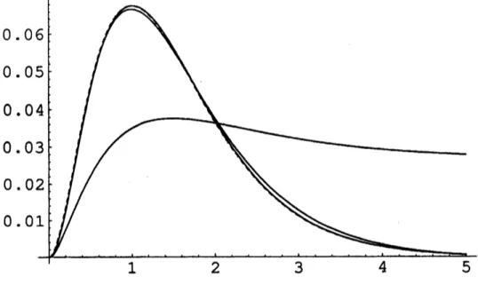
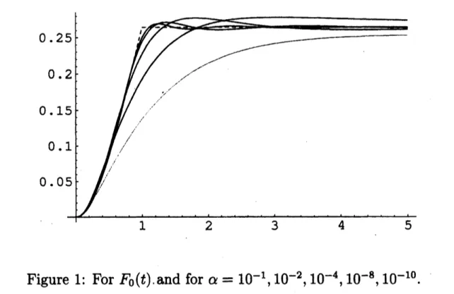
5 Numerical Experiments

We shall give a numerical experiment for the typical example $F_{0}(t)=\{\begin{array}{ll}\text{一} te^{-t}-e^{-t}+1 for 0\leq t\leq 11-2e^{-1} for 1\leq t,\end{array}$

whose Laplace transform is

$( \mathcal{L}F_{0})(p)=\frac{1}{p(p+1)^{2}}[1-(p+2)e^{-(p+1)}]$

.

(5.17)

We set

$g(\xi)=(\mathcal{L}F_{0})(\xi)\xi$

in (3.11) with $(\mathcal{L}K_{\alpha}(\cdot, t))(\xi)\xi=H_{\alpha}(\xi, t)$, then

$F_{\alpha,g}^{*}(t)\sim F_{0}(t)$

(7)

For fixed $t$,

we

calculate the integral (4.16)

over

$[0,50]$ with span

0.01

by

the trapezoidal rule. Here

we

solve the linear simultaneous linear equations

of 5000 by using Matlab. For $t$,

we

take the values

over

$[0,5]$ with span 0.01.

By (3.11),

we

caluculate the inversion by the trapeziodal rule

over

$[0,50]$ with

the span

0.01.

Figure 1: For $F_{0}(t)$.and for $\alpha=10^{-1}$, $10^{-2}$

’ $10^{-4}$’ $10^{-8},10^{-10}$

.

Acknowledgements

Al-Shuaibi visiting Gunma University was supported by the Japan

Coop-eration Center, Petroleum, the Japan Petroleum Institute (JPI) and King Fahd University of Petroleum and Minerals, and he wishes to express his

deep thanks Professor Saburou Saitoh and Mr. Hideki Konishi of the JPI for their kind hospitality. S. Saitoh is supported in part by the Grant-in-Aid for Scientific Research (C)(2)(No. 16540137) from the Japan Society for the Promotion

Science. S.

Saitoh and T. Matsuura

are

partially supported by the Mitsubishi Foundation, the 36th, Natural Sciences, No. 20 (2005-2006).

References

[1] Abdulaziz Al-Shuaibi, On the inversion

_of

the Laplace

_transfom

by $u8e$

of

a

regularized di8placement operator, Inverse Problems 13(1997),

(8)

Figure 2: For $F(t)=\chi(t, [1/2,3/2])$, the characteristic function and for

$\alpha=10^{-1},10^{-4},10^{-8},10^{-12},10^{-16}$

.

$( \mathcal{L}F)(p)=\frac{1}{p}(\exp(-\frac{1}{2}p)-\exp(-\frac{3}{2}p))$

.

Figure 3: For $U(t, [1, \infty])$, the step function and for $\alpha$ $=$

(9)

Figure 4: For $F(t)=1/2t^{2}\exp(-2t)$ and for $\alpha=10^{-1},10^{-4},10^{-8}$

.

$(\mathcal{L}F)(p)=$

$\frac{1}{(p+2)^{3}}$

(10)

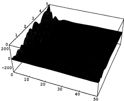
Figure 6: For $H_{\alpha}(\xi, t)$ and for $\alpha=10^{-8}$

.

[2] Abdulaziz Al-Shuaibi, The Riemann zeta

_function

used in the inversion

of

the Laplace transform, Inverse Problems 14(1998), 1-7.

[3] Abdulaziz Al-Shuaibi, Inversion

_of

the Laplace

_transform

via Post-Widder formula, Integral Transforms and Special IFMnctions 11(2001),

225-232.

[4] K. Amano, S. Saitoh and A. Syarif, A Real Inversion Formula

_for

the

Laplace $\pi_{ansform}$ in a Sobolev Space, Z. Anal. Anw. 18(1999),

1031-1038.

[5] K. Amano, _{S. Saitoh}and M. Yamamoto, Error estimates

_of

the real

inver-sion

_fomulas

_of

the Laplace tmnsform, Integral Transforms and Special

IFMnctions, 10 (2000),

_165-178.

[6] A. Boumenir and A. Al-Shuaibi, The Inverse Laplace

_transfo

$7vn$ and

An-alyti$c$

Pseudo-Differential

Opemtors, J. Math. Anal. Appl. 228(1998),

16-36.

[7] D.-W. Byun and S. Saitoh, A real inversion

_formula

_for

the Laplace

(11)

[8] G. Doetsch, Handbuch der Laplace $\mathcal{I}kansformation$, Vol. 1., Birkhaeuser Verlag, Basel,

1950.

[9] H. W. Engl, M. Hanke and A. Neubauer, Regularization ofInverse

Prob-lems, Mathematics and Its Applications 376(2000), Kluwer Academic Publishers.

[10] V. V. Kryzhniy, Regulanized Inversion

_of

Integral $\pi_{a}$

nsformations of

Mellin Convolution $X\mathfrak{y}pe$, Inverse Problems, 19(2003),

1227-1240.

[11] V. V. Kryzhniy, Numerecal inversion

_of

the Laplace

_transfom:

analysis via regulanzed analytic continuation, Inverse Problems, 22 (2006),

579-597.

[12] T. Matsuura and S. Saitoh, Analytical and numerical solutions

_of

lin-ear

ordinary

_differential

equations with constant coefficients, Journal of

Analysis and Applications, 3(2005), pp. 1-17.

[13] T. Matsuura and S. Saitoh, Analytical and numerical real inversion

for-mulas

_of

the Laplace transform, The ISAAC Catani Congress Proceedings

(to appear).

[14] T. Matsuura

and S.

Saitoh,

Analytical

and numerical inversion

_formulas

in the

Gaussian convolution

by using the Paley- Wiener spaces, Applicable Analysis, 85(2006),

901-915.

[15] E. L. Post, Generalized diffentiation, bans. Amer. Math. Soc. 32(1930),

723-781.

[16] S. Saitoh, Integral $I$}_$u$nsforms, Reproducing Kemels and their Applica-tions, Pitman Res. Notes in Math. Series 369, Addison Wesley Longman

Ltd (1997), UK.

[17] S. Saitoh, Approximate real inversion

_{formula8 of}

the Laplace transform, Far East J. Math.

Sci.

11(2003),

53-64.

[18] S. Saitoh, Approvzmate Real Inversion Formulas

_of

the Gaussian

Con-volution, Applicable Analysis, 83(2004), 727-733.

[19] S. Saitoh, Best approvimation, Tikhonov regularization and reproducing

(12)

[20] S. Saitoh, Tikhonov regularization and the theory

_of

reproducing kemels,

Proceedings of the 12th International Conference

on

Finite

or

Infinite

Dimensional Complex Analysis and Applications, Kyushyu University

Press (2005), 291-298.

[21] S. Saitoh, Vu Kim Tuan and M. Yamamoto, Conditional Stability

_of

a Real Inverse Formula

_for

the Laplace $\pi_{ansform}$, Z. Anal. Anw. 20(2001),

193-202.

[22] S. Saitoh, N. Hayashi and M. Yamamoto (eds.), Analytic Extension For-mulas and their Applications, (2001), Kluwer Academic Publishers.

[23] Vu Kim Tuan and Dinh Thanh Duc, Convergence rate

_of

Post- Widder

approximate inversion

_of

the Laplace transform, Vietnam J. Math. 28(2000),

93-96.

[24] Vu Kim Tuan and Dinh Thanh Duc, A

new

real inversion

_{formula for}

the Laplace

_transform

and its convergence $mte$, Rac. Cal.

&Appl.

Anal.

5(2002),

387-394.

[25] D. V. Widder, The inversion

_of

the Laplace integral and the related moment problem, ?kans. Amer. Math. Soc. 36(1934), 107-2000.

[26] D. V. Widder, The Laplace Transform, Princeton University Press, Princeton,

1972.

[27] $http://library$

.

wolfram.

$com/inforcenter/MathSource/4738/$