Numerical
simulation of ffee boundary problems
in
quadruple
precision arithmetic using
explicit
schemes
Dedicated to the sixtieth
birthday
of Professor Hideo Kawarada
HITOSHI IMAI1), YOSHITANE $\mathrm{s}\mathrm{H}\mathrm{I}\mathrm{N}\mathrm{O}\mathrm{H}\mathrm{A}\mathrm{R}\mathrm{A}1$), MAKOTO $\mathrm{N}\mathrm{A}\mathrm{T}\mathrm{O}\mathrm{R}\mathrm{I}^{2}$), WEIDONG ZHOU2), ISAMU $\mathrm{O}\mathrm{H}\mathrm{N}\mathrm{I}\mathrm{S}\mathrm{H}\mathrm{I}^{3}$)
AND YASUMASA NISHIURA4)
1) FacultyofEngineering, University ofTokushima, Tokushima 770, Japan
2) Instituteof Information Sciencesand Electronics, UniversityofTsukuba, Ibaraki 305,Japan
3) Departmentof InformationMathematics, UniversityofElectro-Communications, Tokyo 182, Japan
4) ResearchInstitute for Electronic Science, Hokkaido University, Sapporo 060, Japan
1.
Introduction
Afree boundary problem is
a
problemwhose domain is unknown. Wecan see
manyproblemsin practical phenomenaashee boundary problems. Theyarenonlinear, sonumerical simulations
are inevitable in analysis. Numerical methods for free boundary problems have been developed
and improved, sotheir numerical simulationsarenot
so
difficult recently. However, investigationon reliability of numerical results is not easy. Reliability is usually checked by comparing
nu-merical results obtained in
diffe.rent
precision. In the check distinction between round-offerror
andtruncation
error
is very important. Normal numerical simulationsare
carriedout in doubleprecision arithmetic, soround-off
error can
be reduced by using quadruple precision arithmetic.In the paper
a
numerical method which realize numerical simulations of hee boundary problemsin quadruple precision arithmetic isconsidered.
In numerical simulations FDM or FEM are very popular as descretization methods.
How-ever, changing order is not easy in these methods. Rom this view point spectral methods are
convenient. Numerical methods using spectral collocation methods in space and time
were
de-velopedtoffee boundary$\mathrm{p}\mathrm{r}\mathrm{o}\mathrm{b}\mathrm{l}\mathrm{e}\mathrm{m}\mathrm{S}[2-3]$
.
Inthe methods ordercanbeset easily and $\mathrm{a}\mathrm{r}\mathrm{b}\mathrm{i}\mathrm{t}\mathrm{r}\mathrm{a}\mathrm{r}\mathrm{y}[3]$.
However, the methods
are
implicit in time,so
they need adequate iterative methods and theycost$\mathrm{m}\mathrm{u}\mathrm{c}\mathrm{h}[4]$
.
Thismeans
that theyare
not easily applicable to higher dimensional free boundaryproblems.
In the $\dot{\mathrm{p}}$aper
a
$\mathrm{n}\mathrm{u}\mathrm{m}\mathrm{e}\mathrm{r}\mathrm{i}\mathrm{c}\mathrm{a}\dot{|}1$method to ffee
boundar.y
problems which is explicit in time and2. Numenical
method
2.1.
Higher order
$\mathrm{e}\mathrm{x}\mathrm{p}\mathrm{l}\mathrm{i}_{\mathrm{C}\mathrm{i}\mathrm{t}}$seme
As for accurate simulations of free boundary problems a method which consits of a fixed
domainmethodand spectralcollocation methodsinspaceandtime
was
developed. The methodrealizes arbitrary order in space and $\mathrm{t}\mathrm{i}\mathrm{m}\mathrm{e}[2- 3]$
.
This is advantageous for accuracy. However, itisimplicit in time,so it needs adequateiterarivemethods anditcosts$\mathrm{m}\mathrm{u}\mathrm{c}\mathrm{h}\mathrm{l}4$]. This
means
thatit is not easily applicableto higher dimensional free boundary problems. Hence in the paper an
explicit method is considered.
Here it should be remarked that many time evolutional free boundary problems have time
evolutionalequations of motion of the free boudaries like the Stefan condition. This
means
thatit ispossibletoapplythe Runge-Kutta method. Asis written in theprevioussectionourpurpose
is development of numerical methods for the quadruple precision arithmetic. Therefore, usual
Runge-Kutta methods arenot available. Higher order Runge-Kutta methods are necessary. As
for descretizationinspacespectralcollocation methods
are
used. Theyare
not applicable to freeboundary problems directly. So, a fixed domain method using mapping functions is combined.
The concrete procedure of the above method will be shown in its application to test problems.
2.2. Test
problem
We cosider the following one-dimensional ffee boundary problem as
a
test problem. Thisproblem is related to the free boundary problem describing the pattern formation in diblock
$\mathrm{c}\mathrm{o}\mathrm{p}\mathrm{o}\mathrm{l}\mathrm{y}\mathrm{m}\mathrm{e}\mathrm{r}[6]$
.
Herewe should remark thatour
approach is not limited to this problem.Test Problem(N-N)
:
Find $s(t)$ and $u(x,t)$ such that$\{$ $\frac{d}{dt}s(t)$ $=F(s(t),t)$ $t>0$ $s(0)$ $=- \frac{1}{2}$ where $F(s(t),t)\equiv-u^{+}(xS(t),t)+u_{x}^{-}(S(t),t)$ $\{$
$u_{xx}^{+}(_{X},t)$ $=-2 \frac{t+\frac{11}{4}}{t+2}$ in $(-1, s(t))\mathrm{X}t>0$
$u_{xx}^{-}(_{X,t})$ $=2 \frac{t+\frac{3}{4}}{t+2}$
in $(s(t), 1)\cross t>0$
$u_{x}^{+}(-1,t)$ $=u_{x}^{-}(1,t)=0$ (Neumann-Neumann $\mathrm{B}.\mathrm{C}.$)
for
$t>0$$u^{+}(s(t),t)$ $=u^{-}(s(t),t)=0$
for
$t>0$$\{$
$u^{+}(x, 0)=- \frac{11}{8}(_{X+}\frac{1}{2})(_{X}+\frac{3}{4})$ in $(-1, s(0))$
We also consider two
more
problems Test Problem(N-D) and TestProblem(D-D)by replacing(Neumann-Neumann$\mathrm{B}.\mathrm{C}.$) by the following boundary conditions (Neumann-Dirichlet $\mathrm{B}.\mathrm{C}.$)
or
(Dirichlet-Dirichlet B.C.), respectively.(Neumann-Dirichlet $\mathrm{B}.\mathrm{C}.$):
$u_{x}^{+}(-1,t)$ $=0$
for
$t>0$$u^{-}(1,t)$ $=- \frac{(t+\frac{3}{4})(t+3)^{2}}{(t+2)^{3}}$
for
$t>0$(Dirichlet-Dirichlet $\mathrm{B}.\mathrm{C}.$):
$u^{+}(-1,t)$ $=.. \frac{(t+\frac{11}{4})(t+1)^{2}}{(t+2)^{3}}$
for
$t>0$$u^{-}(1,t)$ $=- \frac{(t+\frac{3}{4})(t+3)^{2}}{(t+2)^{2}}$ $f\sigma r$ $t>0$
Exact solutionsto thesetest problems
are same
and givenas
follows:$\{$
$s(t)$ $=- \frac{1}{t+2}$
for
$t\geq 0$$u^{+}(x,t)$ $=- \frac{t+\frac{11}{4}}{t+2}(x-s(t))(x+2+s(t))$ in $[-1, s(t)]\cross t\geq 0$
$u^{-}(x,t)$ $= \frac{t+\frac{3}{4}}{t+2}(x-s(t))(x-2+s(t))$ in $[s(t), 1]\cross t\geq 0$
2.3.
Fixed domain
method
Descretization in spaceis performed by usingspectralcollocation methods. Here
we
shouldremark that they are applicable only in the interval for one-dimensional problems (or in the
rectangular domain for higher dimensional problems). So they
are
applied after mapping theunknown domainof the problem into the interval [-1, 1] $[2,5]$
.
TestProblems have two intervals$[-1, s(t)]$ and $[s(t), 1]$ separated by the free boundary,
so
these two intervals are mapped into[-1, 1] by different mapping functions. Themappingfunctions
are
givenas
follows:$t=\tau$
for
$\tau\geq 0$$\{$
$x_{\xi}^{+}+\epsilon+(\xi+, \tau)$ $=0$ in $(-1,1)\cross\tau\geq 0$
$x^{+}(-1, \tau)$ $=-.1$
far
$\tau\geq 0$$x^{+}(1, \mathcal{T})$ $=s(\tau)$
for
$\tau\geq 0$$\{$
$x_{\xi^{-\xi}}^{-}-(\xi-, \tau)$ $=0$ in $(-1,1)\cross\tau\geq 0$ $x^{-}(-1, \mathcal{T})$ $=s(_{\mathcal{T})}$
for
$\tau\geq 0$$x^{-}(1, \tau)$ $=1$
Here we should remark that mapping functions on spatial variables
are
givenas
solutions of boundary value problems. This method is called numerical grid$\mathrm{g}\mathrm{e}\mathrm{n}\mathrm{e}\mathrm{r}\mathrm{a}\mathrm{t}\mathrm{i}\mathrm{o}\mathrm{n}[8]$.
These boundaryvalue problems
are
one-dimensional,so
wecan
solve them exactly. However,our
purpose isdevelopment of methods for higher dimensional free boundary problems. Hence we solvethem
numerically. Usingthesemappingfunctions Test Problem(N-N) istransformed intothefollowing
fixed boundaryproblem.
Test Problem(N-N)’
:
$\{$
$\frac{d}{d\tau}s(_{\mathcal{T})} =F(s(\tau), \mathcal{T})$
$s(0)$ $=- \frac{1}{2}$
where
$F(s( \mathcal{T}),t)\equiv\frac{1}{x_{\xi}^{+}(+1,\mathcal{T})}u(\epsilon+1+,)\tau+\frac{1}{x_{\xi^{-}}^{-}(-1,\tau)}u\xi-(--1, \tau)$
for
$\tau>0$$\{$
$\frac{1}{(X_{\xi}^{+})^{2}+}u_{\xi}^{+}+_{\xi}+-\frac{x_{\xi\xi}^{+}++}{(_{X_{\xi}^{+}}+)^{3}}u_{\xi}+=+-2\frac{\tau+\frac{11}{4}}{\tau+2}$ in $(-1,1)\cross \mathcal{T}>0$
$\frac{1}{(X_{\xi^{-}}^{-})^{2}}u^{-}-\frac{x_{\xi^{-\xi^{-}}}^{-}}{(x_{\xi^{-)^{3}}}^{-}}\xi^{-}\xi^{-}\xi u^{-}-=2\frac{\tau+\frac{3}{4}}{\tau+2}$ in $(-1,1)\cross \mathcal{T}>0$
$u_{\xi^{+}\xi^{-(}}^{+}(-1, \tau)=u^{-}1,$$\mathcal{T})=0$
for
$\tau>0$$u^{+}(1, \mathcal{T})=u^{-}(-1, \tau)=0$
for
$\tau>0$$\{$
$u^{+}( \xi^{+,\mathrm{o}})=-\frac{11}{8}(x^{+}(\xi^{+}, 0)+\frac{1}{2})(x^{+}(\xi^{+}, 0)+\frac{3}{4})$ in $(-1, s(0))$
$u^{-}( \xi^{-,\mathrm{o}})=\frac{3}{8}(x^{-}(\xi^{-}, \mathrm{o})+\frac{1}{2})(x^{-}(\xi^{-}, \mathrm{o})-\frac{5}{2})$ in $(s(0), 1)$
We solve this using spectralcollocationmethods in space and the higher order Runge-Kutta
method in time. Test Problems (N-D) and (D-D) are solved in the
same
way.2.4.
Higher order Runge.Kutta method
TheRunge-Kuttamethod isverypopularin numerical computations ofasystem of ordinary
differential equations. Usually the fourth order formula isused, however it is not adequate here.
This is because that our purpose is numerical simulations in quadruple precision arithmetic.
So we use higher order Runge-Kutta methods. There are many $\mathrm{f}_{\mathrm{o}\mathrm{r}\mathrm{m}\mathrm{u}}1\mathrm{a}\mathrm{e}[7]$
.
Here we adoptformulae with the wide stable region and coefficients given by ffactions. The followings
are
formulae used here.
4th order Runge-Kutta method
:
$k_{1}$ $=$
.
$\Delta t\cross F(t_{n}, y_{n})$
$k_{i}$ $=\Delta t\cross F(t_{n}+a(i)\Delta, y_{n}+t_{\dot{\iota}})$ $(i=2, \ldots , 4)$
$y_{n+1}$ $=$ $y_{n}+ \sum_{\dot{\iota}=1}c4(i)k\dot{l}$
where
$a(2)= \frac{1}{2}$ $B(2,1)= \frac{1}{2}$ $B(4,1)=0$ $C(1)= \frac{1}{6}$
$a(3)= \frac{1}{2}$ $B(3,1)=0$ $B(\mathit{4},2)=0$ $C(2)= \frac{1}{3}$
$a(4)=1$ $B(3,2)= \frac{1}{2}$ $B(4,3)=1$ $C(3)= \frac{1}{3}$ $C(4)= \frac{1}{6}$
6th Runge-Kutta method( Verner formula)
:
$k_{1}$ $=$ $\Delta t\cross F(t_{n}, y_{n})$
$t_{i}$ $=$ $\sum_{j=1}^{i-1}B(i, j)kj$ $(\dot{i}=2, \ldots, 8)$
$k_{i}$ $=$ $\Delta t\cross F(t_{n}+a(i)\Delta, y_{n}+t_{i})$ $(i=2, \ldots, 8)$
$y_{n+1}$ $=$ $y_{n}+ \sum_{=i1}^{8}c(i)\dot{k}_{i}$
where
$a(2)= \frac{1}{18}$ $B(2,1)= \frac{1}{18}$ $B(6,1)=- \frac{369}{73}$ $B(8,1)= \frac{3015}{256}$ $C(1)= \frac{57}{640}$
$a(3)= \frac{1}{6}$ $B(3,1)=- \frac{1}{12}$ $B(6,2)= \frac{72}{73}$ $B(8,2)=- \frac{9}{4}$ $C(2)=0$
$a(4)= \frac{2}{9}$ $B(3,2)= \frac{1}{4}$ $B(6,3)= \frac{5380}{219}$ $B(8,3)=- \frac{4219}{78}$ $C(3)=- \frac{16}{65}$
$a(5)= \frac{2}{3}$ $B(4,1)=- \frac{2}{81}$ $B(6,4)=- \frac{12285}{584}$ $B(8, \mathit{4})=\frac{5985}{128}$ $C(4)= \frac{1377}{2240}$
$a(6)=1$ $B( \mathit{4},2)=\frac{4}{27}$ $B(6,5)= \frac{2695}{1752}$ $B(8,5)=- \frac{539}{384}$ $C(5)= \frac{121}{320}$
$a(7)= \frac{8}{9}$ $B(4,3)= \frac{8}{81}$ $B(7,1)=- \frac{8716}{891}$ $B(8,6)=0$ $C(6)=0$
$a(8)=1$ $B(5,1)= \frac{40}{33}$ $B(7,2)= \frac{656}{297}$ $B(8,7)= \frac{693}{3328}$ $C(7)= \frac{891}{8320}$
$B(5,2)=- \frac{4}{11}$ $B(7,3)= \frac{39520}{891}$ $C(8)= \frac{2}{35}$
$B(5,3)=- \frac{56}{11}$ $B(7,4)=- \frac{416}{11}$ $B(5,4)=- \frac{54}{11}$ $B(7,5)= \frac{52}{27}$
$B(7,6)=0$
8th order Runge-Kutta method( Verner formula)
:
$k_{1}$ $=$ $\Delta t\cross F(t_{n},y_{n})$
$t_{i}$ $=$ $\sum_{j=1}^{\dot{\iota}-1}B(i,j)kj$ $(i=2, \ldots , 13)$
$k_{i}$ $=$ $\Delta t\cross F(t_{n}+a(i)\Delta, y_{n}+t:)$ $(i=2, \ldots , 13)$
$y_{n+1}$ $=$ $y_{n}+ \sum_{=i1}^{1}3C(i)k$
:
$a(2)= \frac{1}{4}$ $B(2,1)= \frac{1}{4}$ $B(9,1)= \frac{17176}{25515}$ $B(12,1)=- \frac{27061}{204120}$ $C(1)= \frac{31}{720}$
$a(3)= \frac{1}{12}$ $B(3,1)= \frac{5}{72}$ $B(9,2)=0$ $B(12,2)=0$ $C(2)=0$
$a(4)= \frac{1}{8}$ $B(3,2)= \frac{1}{72}$ $B(9,3)=0$ $B(12,3)=0$ $C(3)=0$
$a(5)= \frac{2}{5}$ $B(.4, 1)= \frac{1}{32}$ $B(9,4)=- \frac{47104}{25515}$ $B(12,4)= \frac{40448}{280665}$ $C(4)=0$
$a(6)= \frac{1}{2}$ $B(4,2)=0$ $B(9,5)= \frac{1325}{504}$ $B(12,5)=- \frac{1353775}{1197504}$ $C(5)=0$
$a(7)= \frac{6}{7}$ $B(4,3)= \frac{3}{32}$ $B(9,6)=- \frac{41792}{25515}$ $B(12,6)= \frac{17662}{15515}$ $C(6)= \frac{16}{75}$
$a(8)= \frac{1}{7}$ $B(5,1)= \frac{106}{125}.$. $B(9,7)= \frac{20237}{145800}$ $B(12,7)=- \frac{71687}{1166400}$ $C(7)= \frac{16807}{79200}$
$a(9)= \frac{2}{3}$ $B(5,2)=0$ $B(9,8)= \frac{4312}{6075}$ $B(12,8)= \frac{98}{225}$ $C(8)= \frac{16807}{79200}$
$a(10)= \frac{2}{7}$ $B(5,3)=- \frac{408}{125}$ $B(10,1)=- \frac{23834}{180075}$ $B(12,9)= \frac{1}{16}$ $C(9)= \frac{243}{1760}$
$a(11)=1$ $B(5,4)= \frac{352}{125}$ $B(10,2)=0$ $B(12,10)= \frac{3773}{11664}$ $C(10)=0$
$a(12)= \frac{1}{3}$ $B(6,1)= \frac{1}{48}$ $B(10,3)=0$ $B(12,11)=0$ $C(11)=0$
$a(13)=1$ $B(6,2)=0$ $B(10,4)=- \frac{77824}{1980825}$ $B(13,1)= \frac{11203}{8680}$ $C(12)= \frac{243}{1760}$
$B(6,3)=0$ $B(10,5)=- \frac{636635}{633864}$ $B(13,2)=0$ $C(13)= \frac{31}{720}$ $B(6,4)= \frac{8}{33}$ $B(10,6)= \frac{254048}{300125}$ $B(13,3)=0$
$B(6,5)= \frac{125}{528}$ $B(10,7)=- \frac{183}{7000}$ $B(13,4)=- \frac{38144}{11935}$
$B(7,1)=- \frac{1263}{2401}$ $B(10,8)= \frac{8}{11}$ $B(13,5)= \frac{2354425}{458304}$
$B(7,2)=0$ $B(10,9)=- \frac{324}{3773}$ $B(13,6)=- \frac{84046}{16275}$
$B(7,3)=0$ $B(11,1)= \frac{12733}{7600}$ $B(13,7)= \frac{673309}{1636800}$ $B(7,4)= \frac{39936}{26411}$ $B(11,2)=0$ $B(13,8)= \frac{4704}{8525}$ $B(7,5)=- \frac{64125}{26411}$ $B(11,3)=0$ $B(13,9)= \frac{9477}{8525}$ $B(7,6)= \frac{5520}{2401}$ $B(11,4)=- \frac{20032}{5225}$ $B(13,10)=- \frac{1029}{992}$
$B(8,1)= \frac{37}{392}$ $B(11,5)= \frac{456485}{80256}$ $B(13,11)=0$ $B(8,2)=0$ $B(11,6)=- \frac{42599}{7125}$ $B(13,12)= \frac{729}{341}$ $B(8,3)=0$ $B(11,7)= \frac{339227}{912000}$ $B(8,4)=0$ $B(11,8)=- \frac{1029}{4180}$ $B(8,5)= \frac{1625}{9408}$ $B(11,9)= \frac{1701}{1408}$ $B(8,6)=- \frac{2}{15}$ $B(11,10)= \frac{5145}{2432}$ $B(8,7)= \frac{61}{6720}$
3.
Numerical results
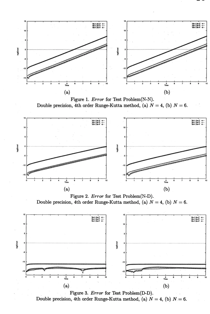
Numerical results to Test Problems $(\mathrm{N}- \mathrm{N}),(\mathrm{N}- \mathrm{D})$ and (D-D) are shownhere. Gauss-Lobatto
collocation points and Chebyshev polynomials
are
used in the spectral collocation $\mathrm{m}\mathrm{e}\mathrm{t}\mathrm{h}\mathrm{o}\mathrm{d}\mathrm{s}[1]$.
Numerical computations are carried out for several orders in spectral collocation methods and
Runge-Kutta methods, in both double and quadruple precision arithmetic. Error $\equiv|S_{exaC}(t)-$
$s_{ca\mathrm{t}(}t)|$ is shown as a function of time $t$, where $s_{exac}(t)$ is an exact solution and $s_{cd}(t)$ is a
computed value. $N+1$ collocation points
are
$\mathrm{u}\mathrm{s}\mathrm{e}\mathrm{d}[1]$.
Numerical computationsare
carried out$\frac{\omega}{\underline 8}\mathrm{H}$
, $\underline{\frac{\omega}{\epsilon}\mathrm{E}}$
(a) (b)
Figure 1. Error for Test Problem(N-N).
Double precision, 4th orderRunge-Kutta method, (a) $N=4,$ $(\mathrm{b})N=6$
.
$\frac{\omega}{\underline s}=\mathrm{g}$ $\frac{\mathrm{u}}{\underline \mathfrak{a}0}\mathrm{t}\succeq$
(a) (b)
Figure 2. Error for Test Problem(N-D).
Double precision, 4th orderRunge-Kutta method, (a) $N=4,$ $(\mathrm{b})N=6$
.
$\frac{\omega}{\underline 8’}=\mathrm{g}$
$\frac{}{\underline 8’}=\frac{\mathrm{e}}{\mathrm{u}}$
(a) (b)
Figure 3. Error for Test Problem(D-D).
$\frac{\mathrm{u}=\mathrm{g}}{\underline 8’}$
$\frac{\mathrm{u}}{\underline 8}=\mathrm{g}$
(a) (b)
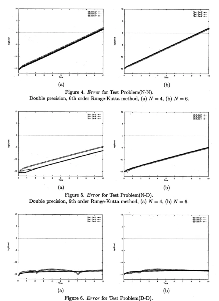
Figure 4. Error for Test Problem(N-N).
Double precision, 6th order Runge-Kutta method, (a) $N=4,$ $(\mathrm{b})N=6$
.
$\frac{\mathrm{u}}{\underline a\mathrm{o}}=_{\mathrm{o}}=$
$\frac{\overline{\overline{\mathrm{u}}}}{\underline@}=0$
(a) (b)
Figure 5. Error for Test Problem(N-D).
Double precision, 6th order Runge-Kutta method, (a) $N=4,$ $(\mathrm{b})N=6$
.
$\frac{\omega}{\underline 8’}=\mathrm{g}$
$\frac{\mathrm{u}}{\underline 8’}=\mathrm{g}$
(a) (b)
Figure6. Error for Test Problem(D-D).
$\dot{\frac{\mathrm{u}}{\mathit{9}}\mathrm{g}}$
$\frac{\omega}{\underline\epsilon}=\mathrm{g}$
(a) (b)
Figure 7. Error for Test Problem(N-N).
Double precision, 8th order Runge-Kutta method, (a) $N=4,$ $(\mathrm{b})N=6$
.
$\underline{=\frac{\omega}{8’}\mathrm{g}}$
$= \frac{\mathrm{u}}{\underline 8}\mathrm{g}$
(a) (b)
Figure 8. Errorfor Test Problem(N-D).
Double precision, 8th order Runge-Kutta method, (a) $N=\mathit{4},$ $(\mathrm{b})N=6$
.
$\frac{\overline{\overline{\omega}}}{\underline \mathrm{P}}=0$
$\frac{}{\underline\epsilon}\frac{\mathrm{E}}{\mathrm{u}}$
(a) (b)
Figure 9. Error for Test Problem(D-D).
$\overline{\frac{\mathrm{u}}{\underline 8’}\overline{\mathrm{g}}}$
$\frac{w}{\underline\epsilon}=\mathrm{g}$
(a) (b)
Figure 10. Error for Test Problem(N-N).
Quadruple precision, 4th order Runge-Kutta method, (a) $N=4,$ $(\mathrm{b})N=6$
.
$\overline{\frac{}{\underline \mathrm{P}}\overline{\frac{arrow}{\mathrm{u}}\circ}}$
$= \frac{\overline{\overline{\omega}}}{\underline@}\mathrm{o}$
(a) (b)
Figure 11. Error for Test Problem(N-D).
Quadruple precision, 4th order Runge-Kuttamethod, (a) $N=4,$ $(\mathrm{b})N=6$
.
$\overline{\frac{\overline{\overline{\mathrm{u}}}}{\underline 8’}\overline{\mathrm{o}}}$ $\frac{}{\underline \mathrm{P}}\frac{\frac{=0}{}}{\omega}$
(a) (b)
Figure 12. Error for Test Problem(D-D).
$\frac{\omega=\mathrm{g}}{\underline\epsilon}$
$\frac{\omega}{\underline\epsilon}\in$
(a) (b)
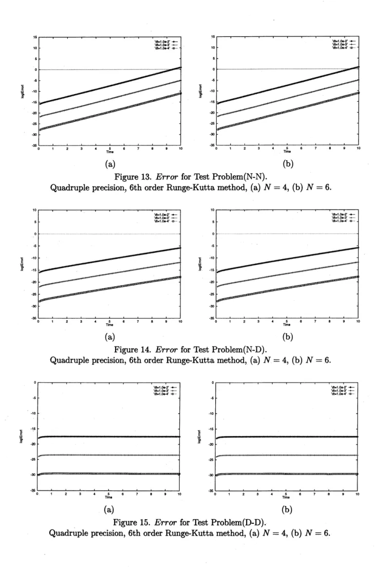
Figure 13. Error for Test Problem(N-N).
Quadruple precision, 6th order Runge-Kutta method, (a) $N=\mathit{4},$ $(\mathrm{b})N=6$
.
$\underline{\frac{\omega}{s}=\mathrm{g}}$ $\frac{}{\underline\epsilon}=\frac{\mathrm{e}}{\mathrm{u}}$
(a) (b)
Figure 14. Error for Test Problem(N-D).
Quadruple precision, 6th order Runge-Kutta method, (a) $N=4,$ $(\mathrm{b})N=6$
.
$\frac{\omega}{\underline 8}=\mathrm{g}$
$\frac{}{\underline\epsilon}=\frac{\mathrm{e}}{\mathrm{u}}$
(a) (b)
Figure 15. Error forTest Problem(D-D).
$\underline{\frac{\omega}{\mathrm{r}\mathrm{o}}=\mathrm{g}}$ $= \frac{\mathrm{u}}{\underline\circ 0}\mathrm{g}$
(a) (b)
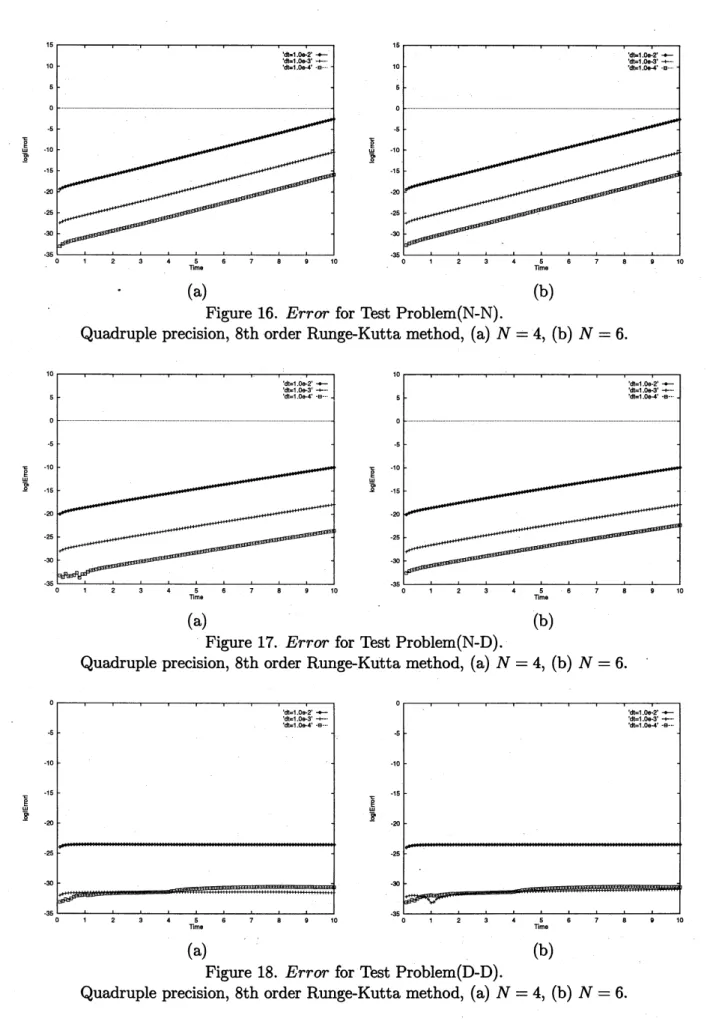
Figure 16. Error for Test Problem(N-N).
Quadruple precision, 8th order Runge-Kutta method, (a) $N=4,$ $(\mathrm{b})N=6$
.
$\frac{\omega}{\underline \mathrm{r}\mathrm{o}}=\mathrm{g}$
(a) (b)
Figure 17. Error for Test Problem(N-D).
Quadruple precision, 8th order Runge-Kutta method, (a) $N=4,$ $(\mathrm{b})N=6$
.
$= \frac{}{\underline 8’}\frac{2}{w}$
$\frac{w}{\underline \mathrm{P}}=\mathrm{g}$
(a) (b)
Figure 18. Error for Test Problem($\dot{\mathrm{D}}$
-D).
Numerical results in double precision arithmetic
are
shown in Figures 1-9. They are almostindependentof$N$becausespatialorderof exactsolutions is low. We
can see
Neumann boundaryconditionsaredelicate in numerical computations. Ifyoudo not haveanyidea insuch situations,
one
answer
isto carry out numerical computations in quadruple precision arithmethic.Numerical results in quadruple precision arithmetic are shown in Figures 10-18. They are
almost satisfactory in accuracy.
\’O
$\mathrm{f}$course
additional considerationsare
necessary ifyou needto carryout longer numerical computations for Nuemann boundary conditions.
4. Conclusion
In the paper a numerical method which is explicit and realize numerical simulations of
fiiee boundary problems in quadruple precision arithmethic is presented. It consists of a fixed
domain method using mapping functions, spectral collocation methods in space and
Runge-Kutta methods in time. For evaluation of
our
method one-dimensional hee boundary problemswhoseexact solutions
are
knownare
solved. Numerical resultsare
satisfactoryinaccuracy. Hereweshould remark that test problems are one-dimensional, however our method is applicable to
higher dimensional free boundary problems.
References
[1] C. Canuto, M.Y. Hussaini, A. Quarteroni and T.A. Zang, “
Spectral Methods in Fluid
Dynamics,”
Springer-Verlag, 1988.[2] H. Imai, Zhou W., M. Natori and H. Kawarada, Numerical Computations of Ihee Boundary
Problems Using the Spectral Method,
“Nonlinear
Mathematical Problems in Industry I $($H. Kawarada et al., eds. ),” Gakuto, 1993, pp.39-47.
[3] H. Imai, Y. Shinohara and T. Miyakoda, Application of Spectral Collocation Methods in
Space and Time to Ree Boundary Problems,
“Hellenic
EuropeanResearch onMathemat-ics and InformatMathemat-ics ’94( E.A. Lipitakis, ed.),” Hellenic Mathematical Society, Vol.2, 1994,
pp.781-786.
[4] H. Imai, Y. Shinohara and T. Miyakoda, On Spectral Collocation Methods in Space and
Time for Free Boundary Problems,
“Computational
Mechanics ’95( S.N.Atluri et al., eds.),” Springer, Vol.1, 1995, pp.798-803.
[5] Y. Katano, T. Kawamura and H. Takami, Numerical Study of Drop Formation ffom a
Capillary Jet Using a General Coordinate System, “
$\mathrm{T}\mathrm{h}\mathrm{e}\mathrm{o}\mathrm{r}\sim \mathrm{e}\mathrm{f}_{\lrcorner}\mathrm{i}_{\mathrm{C}}\mathrm{a}1..\mathrm{a}\mathrm{n}\mathrm{d}$ Applied
Mechanics,”
Univ. Tokyo Press, 1986, pp.3-14.
[6] Y. Nishiura and I. Ohnishi, Some mathematical aspects of the micro-phase separation in
diblock copolymers, Physica D84, 1995, pp.31-39.
[7] M. Tanaka,
“Properties
of the explicit Runge-Kutta $\mathrm{m}\mathrm{e}\mathrm{t}\mathrm{h}_{0}\mathrm{d},$”
Tanaka Lab., Fac. Eng.,
Yamanashi Univ., 1993, in Japanese.
[8] J.F. Thompson,Z.U.A.Warsi andC.W.Mastin, Numerical Grid Generation, North-Holland,