A Single Facility Location Problem with respect to Minisum Criterion II(Optimization Theory and its Applications in Mathematical Systems)

A Single Facility Location Problem with

respect to

Minisum

Criterion

II

Masamichi

Kon $(\Leftrightarrow jE_{1^{\backslash }}\ovalbox{\tt\small REJECT})$

Graduate School

of

Natural

Science and

Technology,

Kanazawa University

Shigeru

Kushimoto $( \bigwedge_{0\backslash }^{\urcorner}\pm* oe)$ Faculty of Education, Kanazawa University

Abstract

The distance (the A-distance) which is determined by given orientations is proposed

by P.Widmayer, Y.F.Wu and C.K.Wong[10]. In this article, we consider a single facility

location problem under the A-distance with respect to minisumcriterion, study properties

of the optimal solution for the problem, and propose “TheIterative Algorithm” to find $aU$

optimal solutions. In $R^{2}$, we consider the problem

$\min_{X\in R^{2}}F(x)=\sum_{i=1}^{n}w_{i}d_{A}(x,y_{i})$,

where$d_{A}$ isthe A-distance.

For each demand point and each givenorientation, we draw a oriented line which passes

the point. Then a plane is divided into regions. We call a point passing some lines an

intersectio$npo$int. Itis shown that there exists anoptimalsolution in theset of intersection

$po$ints. Let$P$be thesmallest convex polygon including ffi demand points, which all boundary

lines are givenorientatedlines. It is shown that any optimaJ solution is in$P$

.

Wepropose “TheIterativeAlgorithm”, where the solutionin eachstep is an interseciion

$po$int. This algorithmisas follow$s$: We choose any demand point as aninitial solution. The

solution in the next step is determined as the adjacent intersection $po$int in the steepest

orientation among orientations accordingtolines which passesthepresent solution. Wealso

proposethe method todetermine the adjacent intersectio$n$ pointeasily by sorting lines.

Keywords : Location problem, Minisumcriterion, A-metric, A-distance

1

Introduction

When we consider wheie a facility should be located on a plane, the problem will be a single

facihty location problem. In this paper, we assume that the facihty can be located almost

everywhere on a plane. Such a model is called a continuous model. We use minisum criterion. For example, minisum criteiion is used when the facihty is the public one. In this article,

we consider a single facihty location problem of a continuous model with respect to minisum criterion.

On the other hand, the location problem is different accoiding to the distance used in it. So various distances are used [1,2,6,7,8,9]. The distance (the A-distance) which is determined

by given orientations is proposed by P.Widmayer, Y.F.Wu and C.K.Wong[10]. We consider the above location problem under the A-distance.

Insection2,we givesomedefinitions and iesults for the A-distance. In section3, we formulate a single facihty minisum location problem under the A-distance, and give some properties of the optimal solution, and propose an iterative algorithm for that problem.

2

The

A-Metric

In $R^{2}$, let

$A=\{\alpha_{1}, \alpha_{2}, \cdots, \alpha_{m}\},$ $m\geq 2$

be a set of given orientations, where $\alpha i$’s are angles for positive direction of x-axis, and we

assume that $0\leq\alpha_{1}<\alpha_{2}<\cdots<\alpha_{m}<\pi$.

If the orientation of a line (a half line, a line segment) belongs to $A$, we call the line (the

halfline, the line segment) A-oriented line (half line, line segment).

Let $B=$

{

$L$ : A-oriented line segment}, and for _{$x_{1},$}$x_{2}\in R^{2}$, let $[x_{1}, x_{2}]=\{x=\lambda x_{1}+(1-$

$\lambda)x_{2}:0\leq\lambda\leq 1\}$. The A-distance is defined as follows.

Deflnition 1 (The A-Distance) For any $x_{1},$$x_{2}\in R^{2}$, we

define

the A-distance between $x_{1}$ and $x_{2}d_{A}(x_{1}, x_{2})$ as

$d_{A}(x_{1}, x_{2})=\{\begin{array}{ll}d_{2}(x_{1}, x_{2}), [x_{1}, x_{2}]\in B\min_{x_{3}\in R^{2}}\{d_{2}(x_{1}, x_{3})+d_{2}(x_{3}, x_{2})|[x_{1}, x_{3}], [x_{3}, x_{2}]\in B\}, oth erwise\end{array}$

where $d_{2};_{S}$ the Euclidean metric. We call $d_{A}$ the A-metric, Infact, $d_{A}$ is a metric in $R^{2}[10]$.

Theorem 1 ([10]) For any $A$ and any $x_{1},$$x_{2}\in R^{2},$ $d_{A}(x_{1}, x_{2})$ is always realized by the

polyg-onal line which consists

_of

at most two A-oriented $\dot{l}$ne segments,

In the following, we assume that $A$ is given.

Definition 2 (The A-Circle) For a point $y\in R^{2}$ and a constant $c>0$,

$\{x\in R^{2}|d_{A}(y, x)=c\}$

is called the A-circle with radius $c$ at center _$y$

.

For the simplicity, let $\alpha_{m+k}=\pi+\alpha_{k}(k=1,2, \cdots, m)$and$\alpha_{0}=\alpha_{2m}-2\pi,$ $\alpha_{2m+1}=\alpha_{1}+27\Gamma$.

In this case, it follows that $0\leq\alpha_{1}<\alpha_{2}<\cdots<\alpha_{m}<\pi\leq\alpha_{m+1}<\cdots<\alpha_{2m}<2\pi$. Moreover,

let $a_{j}=(\cos\alpha_{j}, \sin\alpha_{j})(j=0,1, \cdots, 2m+1)$.

Figure 1.

By Definition 1, we can show the following lemmaeasily.

Lemma 1 ([6]) For $x$ $=$ $(x^{1}, x^{2}),$ $y$ $=$ $(y^{1}, y^{2})$ $\in$ $R^{2}$,

if

$x$ $\in$ $y+C\{aa\}$, where

$C\{a_{j}, a_{j+1}\}=\{\lambda a_{j}+\mu aj+1|\lambda, \mu\geq 0\}$, then $d_{A}(x, y)$ can be represented as

follows.

(2.1) $d_{A}(x, y)= \frac{(x^{1}-y^{1})(\sin\alpha_{j+1}-\sin\alpha_{j})+(x^{2}-y^{2})(\cos\alpha-\cos\alpha)}{\sin(\alpha j+1-\alpha j)}$ Lemma 2 ([6]) For each$y\in R^{2},$ _{$f(x)=d_{A}(x, y)$} is a convexfunction,

3

The

Minisum Location

Problem

In this section, we consider a single facihty minisum location problem under the A-distance. In $R^{2}$, let _{$y_{i}=(y^{i}, y_{1}^{2})$} {or $i=1,2,$

$\cdots,$$n$, be the location of$n$ demand points, $wi$ be positive

weight associated each demand point $i,$ $x$ be the location of the facihty to be located. The

problem is formulated as follows.

(3.1) $\min F(x)$

$x\epsilon R^{2}$

where $F(x)= \sum_{i=1}^{n}w:d_{A}(x, y_{i})$

.

By Lemma 2, $F$ is a convexfunction. Therefore, (3.1) is the convex programming problem.

Furthermore, there exists an optimal solution for (3.1). Let $S^{*}$ be a set of optimal solutions for (3.1).

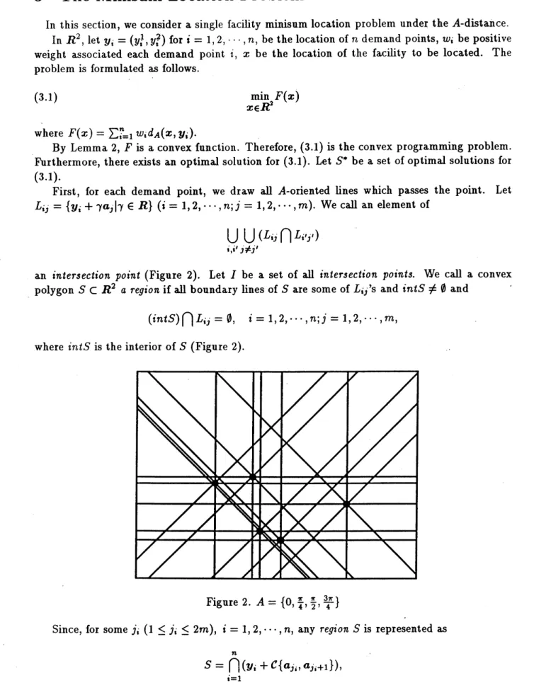
First, for each demand point, we draw $aU$ A-oriented lines which passes the point. Let $L_{1j}=\{y_{i}+\gamma aj|\gamma\in R\}$ $(i=1,2, \cdots, n;j=1,2, \cdots , m)$. We call an element of

$| \bigcup_{1’j}\bigcup_{\neq j’}(L_{1j}\cap L_{i’j’})$

an intersection point (Figure 2). Let $I$ be a set of all intersection points. We call a convex

polygon $S\subset R^{2}$ a region if $aU$ boundary lines of $S$ are some of $L_{1j}$’s and $intS\neq 1$ and

$(intS)\cap L_{ij}=\emptyset$, $i=1,2,$$\cdots,$$n;j=1,2,$$\cdots,$$m$,

where intS is theinterior of $S$ (Figure 2).

Figure 2. $A= \{0, \frac{\pi}{4}, \frac{\pi}{2}, \frac{3\pi}{4}\}$

Since, for some $j;(1\leq j;\leq 2m),$ $i=1,2,$$\cdots,$ $n$, any region $S$ is represented as

$F$ is linear on each region $S$ by (2.1). On the other hand, for any $x \not\in\bigcup_{i,j}L_{ij}$, the region $S$

whose interior contains $x$ is determined uniquely as follows.

$S= \bigcap_{1=1}^{n}(y_{i}+C\{a_{g:}, a_{J;+1}\})$

where

$x\in y_{i}+C\{a:’ a\}$, $i=1,2,$$\cdots,$ $n$

.

In this case, we $caU$ the region $S$ the region characterized by $x$, and write $S(x)$

.

Theorem 2

$S^{*}\cap I\neq\emptyset$

Theorem 3 Let$S_{1},$ $S_{2}$ be adjacent bounded regions.

$S_{1}\subset S^{*}\Rightarrow S^{*}\cap(intS_{2})=\emptyset$

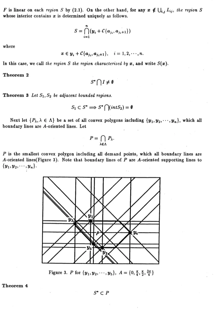
Next let $\{P_{\lambda}, \lambda\in\Lambda\}$ be a set of $aU$ convex polygons including $\{y_{1}, y_{2}, \cdots, y_{n}\}$, which all

boundary lines are A-oriented lines. Let

$P= \bigcap_{\lambda\in\Lambda}P_{\lambda}$.

$P$ is the smallest convex polygon including $aH$ demand points, which all boundary lines are

A-oriented lines(Figure 3). Note that boundary lines of $P$ are A-oriented supporting lines to $\{y_{1}, y_{2}, \cdots,y_{n}\}$

.

Figure 3. $P$ for $\{y_{1}, y_{2}, \cdots, y_{5}\},$ $A= \{0, \frac{\pi}{4}, \frac{\pi}{2}, \frac{3\pi}{4}\}$

Theorem 4

By Theorem 2 and 4, there exists an optimal solution which is an intersection point on

$P$

.

So we consider to deteimine such an optimal solution by iteiative method that traces only

iniersection points where a initial point is any demand point. Now we assume that a solution after the rth iteration is $x^{(r)}$

.

Of cource, $x^{(r)}\in I$

.

We say $a_{j}(1\leq j\leq 2m)$ holds condition (Q) for $x^{(r)}$ if

$\exists y_{i}(1\leq i\leq n)$ s.t. $y_{i}=x^{(r)}+\gamma aJ$ for some $\gamma\in R$

and

$\exists\epsilon>0$s.t. $x^{(r)}+\epsilon a4\in P$

.

Let

$J=$

{

$j|aj$ holds condition (Q) for $x^{(r)}$

}.

For the objective function $F$, we represent the right differential coefficient of $F$ at $x_{0}\in R^{2}$

with respect to $0\neq a\in R^{2}$ as $\partial_{+}F(x_{0};a)$, andlet

(3.2) $u^{(r)}= \min_{j\in J}\{a)\}$.

If $u^{(r)}\geq 0$ then $x^{(r)}$ is optimal by the convexity of the objectivefunction $F$

.

By Theorem 3 and 4, the set of optimal solutions $S^{*}$ is an intersection point or A-oriented line segment, whose end points are adjacent intersec tion points, or a region.

Before we state the algorithm, we consider the determination of $P$

.

First, we sort $L_{ij}$’s

accordingto x-interceptor y-intercept. For each$j$, if$\alpha_{j}\neq\frac{\pi}{2},$$L_{lj}$ is $-x\tan\alpha_{J}\cdot+y=y_{i}^{2}-y_{t}^{1}\tan\alpha_{J}\cdot$,

let $b_{tj}=y_{i}^{2}-y_{i}^{1}\tan\alpha_{j}$. Otherwise, i.e. $\alpha_{j}=\frac{\pi}{2},$ $L_{ij}$ is $x=y_{1}!$, let $b_{tj}=y_{\iota}^{i}$

.

For each $j$, we sort all differentlines among $L_{ij},$ $i=1,2,$$\cdots,$ $n$ according to $b_{ij},$ $i=1,$$\cdots$,$n$

in ascending order. Let those lines be $l_{1}^{j},\ell_{2}^{j},$

$\cdots,l_{n;}^{j}$, where $l_{i}^{j}$ is the ith line among

$\alpha 4$-oriented

soited lines. Note that $n_{j}\leq n$

.

Now we assume that $0\leq\alpha_{1},$$\cdots,$$\alpha_{q-1}<\frac{\pi}{2},$ $\alpha_{q}=\frac{\pi}{2},$ $\frac{\pi}{2}<\alpha_{q+1},$ $\cdots,$$\alpha_{m}$

.

Next we arrange $\ell_{i}^{j},$ $i=1,2,$

$\cdots,$$nj;j=1,2,$$\cdots,$$m$ as follows.

(3.3) $\ell_{1}^{1},$$l_{1}^{2},$

$\cdots,$$\ell_{1}^{q-1},l_{n_{q}}^{q},\ell_{n_{q+1}}^{q+1},$ $\cdots,$$l_{n_{m}}^{m},$ $l_{n_{1}}^{1},\ell_{n}^{2_{2}},$$\cdots,$$\ell_{n_{q-1}}^{q-1},l_{1}^{q},$$l_{1}^{q+1},$_$\cdots,$$l_{1}^{m}$

Now coefficients of$L_{ij}$’s are stored. When we consider $P,$ $=$” in $\ell_{1}^{J}(1\leq j\leq m)$ is replaced by

$\geq$”, and $=$” in $\ell_{n}^{j}j(1\leq j\leq m)$ is replaced by $\leq$”. $P$is the region determined by its system

of inequalities. Note that this system of inequalities may contain reduntant inequalities.

For the simplicity of the representation, let lines in (3.5) be $\ell(1),$ $\ell(2),$_$\cdots,$$\ell(2m)$

.

Especially, let $\ell(2m+1)=\ell(1),$$l(2m+2)=\ell(2)$

.

The procedure for the determination of$P$

Step 1. Determine an intersection point of$l(1)$ and $l(2)$, and let its intersection point be $z_{1}$

.

Set $j=2$

.

Step 2. Determine an intersection point of$\ell(j)$ and $\ell(j+1)$, and let its intersection point be $z_{j}$

.

Step 3. If_$zj=zj-1$ then remove $\ell(j)$

.

Let $l(j_{1}),$ $l(j_{2}),$ $\cdots,$ $l(j_{p})$ be lines left after the above proceduie. $P$ is repiesented by

the system of inequalities corisponding to those lines. Now its system ofinequalities does not

contain iedundant inequalities.

The Iterative Algorithm

Step 1. Choose any demmd point as an initial solution $x^{(0)}$

.

(We choose the demand point

with thelaigest weight.) Set $r=0$

.

Step 2. Calculate $u^{(r)}$

.

Step 3. If$u^{(r)}>0$ _{then stop.} $x^{(r)}$ is an optimal solution.

Step 4. If$u^{(r)}=0$_{then stop. If thenumbei of}$a_{k}$’s whichhold $u^{(r)}=0$, i.e. $\partial_{+}F(x^{(r)};a_{k})=0$,

is

1. one, then any point on$[x^{(r)}, x_{k}^{(r)}]$, where $x_{k}^{(r)}$ is an

$a_{k}$-oriented adjacentitintersection

point to $x^{(r)}$, is optimal.

2. two, then for sufficiently small $\epsilon>0$ and $a_{k_{1}},$$a_{k_{2}}$ which hold $u^{(r)}=0$, any point

$x\in S(x^{(r)}+\epsilon(a_{k_{1}}+a_{k_{2}}))$is optimal.

Step 5. Otherwise, i.e. $u^{(r)}<0$_{, choose any} $a_{k}$ which holds $u^{(r)}=\partial_{+}F(x^{(r)};a_{k})$, and let

$x^{(r+1)}$ be an

$a_{k}$-oriented adjacent intersection point to $x^{(r)}$

.

Set $r=r+1$, and go to Step 2.

The Iterative Algorithm is convergent because $x^{(r)}$ in The Iterative Algorithm is different

from $x^{(0)},$ $x^{(1)},$

$\cdots,$$x^{(r-1)}$ and the numbei of intersection points is finite. Since the number of

intersection poins is $\mathcal{O}(n^{2})$ andthe complexity ofcaluculation of$F(x^{(r)})$is$\mathcal{O}(n)$, the complexity ofThe Iterative Algorithm is $\mathcal{O}(n^{3})$

.

If $ak$ which holds $u^{(r)}=\partial_{+}F(x^{(r)};ak)$ is deteimined in Step 5 of The Iterative Algorithm,

we need to determine $x^{(r+1)}$ _which is an

$a_{k}$-oiiented adjacent intersection point to $x^{(r)}$

.

Next

we consider the piocedure to determine $x^{(r+1)}$

.

For _each $j$, let $f_{j}(x, y)$ be the left side of $L_{tj}$,

i.e.

$f_{j}(x, y)=\{\begin{array}{ll}-x\tan\alpha j+y if \alpha_{j}\neq\frac{\pi}{2},x if \alpha j=\frac{\pi}{2}.\end{array}$

If$\alpha J\neq\frac{\pi}{2}$ then $\nabla f_{j}(x, y)=(-\tan\alpha j, 1)$ otherwise $\nabla f_{j}(x, y)=(1,0)$

.

We assume that an initial solution $x^{(0)}=y_{i_{0}}$ is given. Set $r=0$ wheie $r$ is a counter. Next,

we determine

$p_{s_{r}(j)},$ $j=1,2,$$\cdots,$$m;1\leq s_{r}(j)\leq n_{j}$

coiresponding to $L_{t_{0}}j,$ $j=1,2,$$\cdots,$$m$ (e.g. binary search). Note that $x^{(r)}$ is an intersection

pointof$l_{s_{r}(j)}^{j}\prime s$, i.e. $x^{(r)}$ can be representedby $s_{r}(j)’ s$

.

Weconcentrate on $s_{r}(j),$ $j=1,2,$_$\cdots,$$m$

.

We assume that $\alpha_{k}(1\leq k\leq 2m)$ is determined in Step 5 ofThe Iterative Algoiithm. Let

$j’=\{\begin{array}{ll}k if 1\leq k\leq m,k-m if m<k\leq 2m.\end{array}$

For $j\neq k,$$j\neq k-m(1\leq j\leq m)$, let

where $<x,y>$ is innei product of$x,$ $y\in R^{2}$

.

Next, {oreach$j\neq j’(1\leq m)$, we determine an intersection pointof$\ell_{s_{r}(j)}^{j’}$ and$l_{s_{r}(j)+sign(t_{kj})}^{j}$,

where, for $x\neq 0$,

sign$(x)=\{\begin{array}{l}+1 if x>0,-1 if x<0.\end{array}$

For $j\neq j’(1\leq j\leq m)$, let $z_{kj}$ be an intersection point of

(3.4) $l_{s_{r}(j)}^{j’}$ and $\ell_{s_{r}(j)}^{j}$

.

$z_{kj}$’s are candidates for $x^{(r+1)}$

.

Let

(3.5) $J^{(r)}= \{j:d_{2}(x^{(r)}, z_{kj})=\min_{i\neq j,1\leq i\leq m}\{d_{2}(x^{(r)}, z_{kj})\}\}$

.

$x^{(r+1)}$ is an intersection point of$\ell_{s_{\Gamma}(j)+sign(t_{kj})}^{j},$ $j\in J^{(r)}\cup\{j’\}$

.

Let

(3.6) $s_{r+1}(j)=\{\begin{array}{ll}s_{r}(j) if j=j’,s_{r}(j)+sign(t_{kj}) if j\in J^{(r)},s_{r}(j)+0.5sign(t_{kj}) otherwise.\end{array}$

Set $r=r+1$, and go to the next step.

In the next step, a solution$x^{(r)}$ is an intersection pointof$l_{s_{r}(j)}^{j}$’s such that $s_{r}(j)\in N$ where

$N$is aset ofnatural numbers. For $j$ such that $s_{r}(j)\not\in N$, it means that $x^{(r)}$ lies between $l^{j}$

$[s_{r}(j)]$

and $l_{[s_{r}(j)]+1}^{j}$ where $[\cdot]$ is Gauss’ symbol.

InTheIterativeAlgorithm, wecondider therepresentation ofasolution after the rth iteration

$x^{(r)}$ as

$x^{(r)}\ell^{j}$,

$s_{\Gamma}(j)j=1,2,$$\cdots,$$m$.

The above is only the case of $r=0$. If we consider the case of $r\geq 1$ in The Iterative Algorithm, sign$(t_{kj})$ in (3.4) and the second equation in (3.6) is replaced by

$[s_{r}(j)-0.5]$ if sign$(t_{kj})=-1$,

$[s_{r}(j)+1]$ ifsign$(t_{kj})=1$,

and sign$(t_{kj})$ in the third equation in (3.6) is replaced by

sign$(t_{kj})([s_{r}(j)]-[s_{r}(j)-0.5])$.

4

Numerical

Example

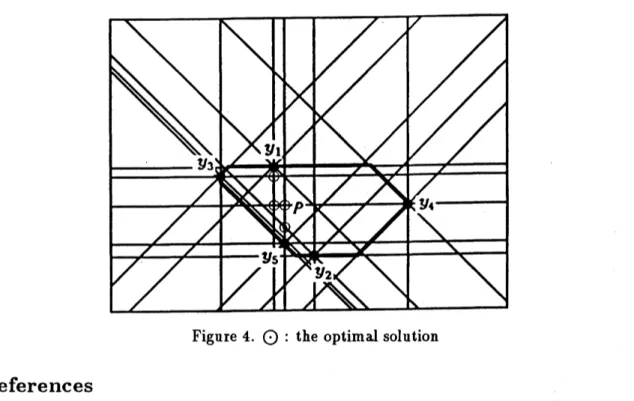
In the problem (2), let $n=5,$$A= \{0, \frac{\pi}{4}, \frac{\pi}{2}, \frac{3\pi}{4}\},$ $y_{1}=(63,97),$ $y_{2}=(102,7),$$y_{3}=(10,90),$_{$y_{4}=$}

$(197,57),$$y_{5}=(73,20),$$w_{1}=w_{2}=w_{3}=w_{4}=w_{5}=1$

.

We set $x^{(0)}=y_{1}$ as an initial solution,

(73,57),$x^{(4)}=$ $($73,36). The optimal solution is $x^{(4)}=$ (73,36), and the optimal value is

$F(x^{(4)})=340.22$ _{(Figure 4).}

Figure 4. : the optimal solution

References

[1] Z.Drezner and A.J.Goldman, “On the Set of Optimal Points to the Weber Problem”,

Trans. Sci., Vol.25, No.1, 1991, 3-8

[2] Z.Drezner and G.O.Wesolowsky, “The Asymmetric Distance Location Problem”, Trans. Sci., Vol.23, No.3, 1989, 201-207

[3] H.Konno and H.Yamashita, “Nonlinear Programming (in Japanese)”, Nikkagiren, Japan,

1978

[4] S.Kushroto, “The Foundations for the optimization (in Japanese)”, Morikita Syuppan,

Japan, 1979

[5] R.T.Rockafellar, “Convex Analysis”, Princeton University Press, Princeton,N.J., 1970 [6] S.Shiode and II.Ishii, “A Single Facihty Stochastic Location Problem under A-Distance”,

Ann. Oper. Res., Vol.31, 1991, 469-478

[7] J.E.Ward and R.E.Wendell, “Using Block Norms for Location Modeling”, Oper. Res., Vol.33, 1985, 1074-1090

[8] J.E.Ward and R.E.Wendell, “A New Norm for Measuring Distance Which Yields Linear Location Problems”, Oper. Res., Vol.28, No.3, 1980, 836-844

[9] R.E.Wendell, A.P.Hurter, Jr. and T.J.Lowe, “Efficient Pointsin Location Problems”, AIIE

Trans., Vol.9, No.3, 1977, 238-246

[10] P.Widmayer, Y.F.Wu and C.K.Wong, “On Some Distance Problems in Fixed