Chaos and relative entropy

(1)

Chaos and relative entropy

Author Yuya O. Nakagawa, Gabor Sarosi, Tomonori Ugajin

journal or

publication title

Journal of High Energy Physics

volume 2018

number 2

year 2018‑07‑02

Author's flag publisher

URL http://id.nii.ac.jp/1394/00000814/

doi: info:doi/10.1007/JHEP07(2018)002

(2)

JHEP07(2018)002

Published for SISSA by Springer Received: June 1, 2018 Accepted: June 22, 2018 Published: July 2, 2018

Chaos and relative entropy

Yuya O. Nakagawa,â Gábor Sárosi^b,c and Tomonori Ugajin^d

aInstitute for Solid State Physics, the University of Tokyo, Kashiwa, Chiba 277-8581, Japan

bDepartment of Physics and Astronomy, University of Pennsylvania, 209 South 33rd Street, Philadelphia, PA 19104-6396, U.S.A.

cTheoretische Natuurkunde, Vrije Universiteit Brussels, Pleinlaan 2, Brussels, B-1050, Belgium

dOkinawa Institute of Science and Technology,

Tancha, Kunikashira gun, Onna son, Okinawa 1919-1, Japan

E-mail: [email protected],[email protected], [email protected]

Abstract: One characteristic feature of a chaotic system is the quick delocalization of quantum information (fast scrambling). One therefore expects that in such a system a state quickly becomes locally indistinguishable from its perturbations. In this paper we study the time dependence of the relative entropy between the reduced density matrices of the thermofield double state and its perturbations in two dimensional conformal field theories. We show that in a CFT with a gravity dual, this relative entropy exponentially decays until the scrambling time. This decay is not uniform. We argue that the early time exponent is universal while the late time exponent is sensitive to the butterfly effect. This large c answer breaks down at the scrambling time, therefore we also study the relative entropy in a class of spin chain models numerically. We find a similar universal exponential decay at early times, while at later times we observe that the relative entropy has large revivals in integrable models, whereas there are no revivals in non-integrable models.

Keywords: AdS-CFT Correspondence, Quantum Dissipative Systems, Conformal Field Theory

ArXiv ePrint: 1805.01051

(3)

JHEP07(2018)002

Contents

1 Introduction 2

2 Localized perturbations 6

2.1 General replica setup 6

2.1.1 Smalllimits 8

2.1.2 Chaos and the late time limit 9

2.2 The modular Hamiltonian part 10

2.3 The entanglement entropy part in general 13

2.4 The entanglement entropy part from large cvacuum block 15

3 Discussion of the result 16

3.1 Timescales in the largec Virasoro answer 16

3.2 Relative entropy and the chaos bound 17

3.3 Comment on integrable systems 19

3.4 The t_W dependence 20

4 Holographic calculation I: global shocks 21

4.1 Dual geometries 22

4.2 Holographic calculations of the entanglement entropy 23

4.3 Evaluation of modular Hamiltonian part 23

4.4 Relative entropy 24

5 Holographic calculations II: localized shocks 24

5.1 Dual gravity geometry 25

5.2 The geodesic length 25

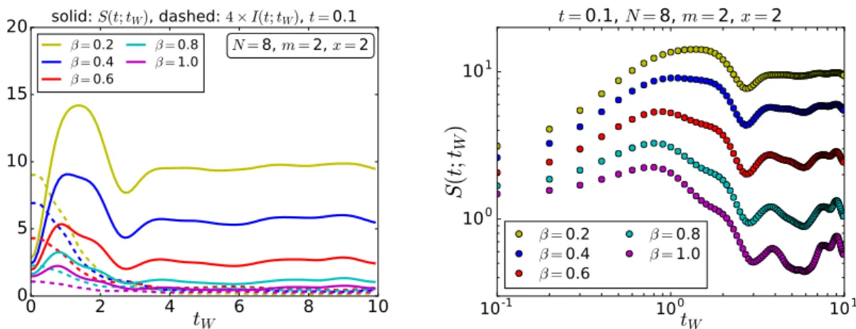
6 Spin chains 26

6.1 Setup of spin chain 26

6.2 t-dependence of the relative entropy 27

6.3 t_W-dependence 27

7 Discussions 29

A The out of causal contact case for localized perturbations 30 B Relative entropy between two perturbed states 32

C Relative entropy of two disjoint intervals 33

C.1 Holographic entanglement entropy 33

C.2 Modular Hamiltonian of the TFD state for two disjoint intervals 34

C.3 Relative entropy 36

(4)

JHEP07(2018)002

1 Introduction

There are many different notions of chaos with a somewhat limited understanding of the relation between them. Some of these are

1. For classical systems, under chaos we usually mean some notion of ergodicity of the dynamics. One signal of ergodicity is chaotic mixing of phase space trajectories, which is related to the heavy dependence of them on small perturbations of the initial conditions [1]. This is called the butterfly effect and is characterized by a so called Lyapunov exponentλ_L, setting the speed at which nearby trajectories diverge at early times.

2. For quantum systems, there is a notion of thermalization, which means that simple (time ordered) correlators relax to their thermal values if the system is started from some non-equilibrium state. This is an early time effect that happens at times of order β=T⁻¹, where T is the temperature.

3. For quantum systems with a classical limit controlled by some tuneable parameterχ, the classical butterfly effect is related to the exponentially decaying behaviour of out of time order correlators (OTOC) [2] at times smaller than the so called Ehrenfest time t_E = _λ¹

Llog_χ¹ [3]. For general quantum systems, the OTOCs can still have Lyapunov type behaviour and the rate of their decay is bounded as λL ≤ 2πT /~

because of causality and unitarity constraints [4]. The Lyapunov behaviour happens at intermediate time scales, which are much longer than the thermalization time.

Note that χ might be~ in which case the bound is trivial in the classical limit, but this is not necessary. For example, in AdS/CFT one has χ=N⁻².

4. Another, intrinsically quantum notion of chaos is the randomness of the energy spectrum, more precisely, the level spacing statistics, which is said to be chaotic if it agrees with that of random matrix theory [5], in particular when nearby energy lev- els repel each other [6, 7]. Since this phenomenon is sensitive to the discreteness of the spectrum, it is associated to effects at very late times, exponential in the entropy.¹ 5. For quantum systems with some locality structure, there are notions like the eigen- state thermalization hypothesis, which is the statement that energy eigenstates appear thermal when probed by sufficiently simple and local probes [9–11].

6. Again for quantum systems with a notion of locality, there is the phenomenon of scrambling of localized quantum information [12]. At the intuitive level, this is related to classical notions of ergodicity and divergence of trajectories, as both these measure how mixing the dynamics is, and how much it forgets about initial conditions. There is both the question of the speed of scrambling (measured by some scrambling time) and how effectively does it happen, i.e. how scrambled localized information can get. There are many quantities sensitive to this type of physics. For example, the

1See also [8] in the context of black holes.

(5)

JHEP07(2018)002

previously mentioned OTOCs are also sensitive to this at late times, because they can be regarded as simple measures of operator growth in the sense of Lieb-Robinson bounds [13–16].² Beyond this, quantum information theoretic quantities, like the trace distance [17], the mutual information or the tripartite information [18] are also sensitive to scrambling.

The primary aim of this paper is to add another quantity to points 3and 6, which is sensitive to scrambling and possibly the Lyapunov behaviour, namely the relative entropy of reduced density matrices associated with a local subregion. The relative entropy S(ρ||σ) measures the distinguishability of two density matrices ρ and σ, and is defined by³

S(ρ||σ) = trρlogρ−trρlogσ. (1.1) Note thatS(ρ||σ) = 0 impliesρ=σ. When a system scrambles, i.e. quantum information becomes quickly delocalized, the reduced density matrices ρ_φ, ρ_ψ of two states |φi,|ψi of similar energy become hardly distinguishable after the scrambling time without having access to a large fraction of all the degrees of freedom. Based on this, we expect the relative entropy on a spatial subsystem to show a decaying behaviour, with the rate of the decay quantifying the speed of scrambling, while the late time value, after the decay ends, quantifying how scrambled the initially localized information can get. In a chaotic system, we therefore expect this late time value to be small.⁴

To sharpen this intuition, we could think about scrambling as the question of how effectively can we recover information from a state after the application of a quantum channel N_t which consists of time evolution followed by a partial trace over some spatial region B

ρ7→ N_t(ρ) = Tr_B e^−iHtρe^iHt

. (1.2)

For such noninvertible channels, there exist approximate recovery maps. However, the possible effectiveness of such recovery channels is bounded by the relative entropy [32]⁵

S(ρ||σ)−S(N_t(ρ)||N_t(σ))≥ −2 logF(ρ,Rσ,N_t(ρ)), (1.3) whereρ andσ are any two states and R_σ,N_t is a particular approximate recovery channel which can recover the stateσ, whileF is the fidelity. In this sense, the time dependent relative entropyS(N_t(ρ)||N_t(σ)) tells us how quickly approximate recovery from this channel can fail.

2While OTOCs are always sensitive to scrambling, the classical butterfly effect, mentioned in point3, only makes sense if there is a classical limit of the system. It is not entirely clear what is the precise connection between these two types of physics, in particular notions like the scrambling time (the time when initally localized information gets maximally scrambled) and the Ehrenfest time (the time when a wavepacket spreads so much that the classical approximation breaks down). In holographic systems, the two timescales are the same basically because the parameter controlling the classical limit is also related to the number of degrees of freedom. In a generic system with a classical limit such relation does not necessarily exist.

3The relative entropy has been used efficiently in the recent quantum information theoretic approach to some fundamental questions in quantum field theory [19–23] and quantum gravity [24–30].

4Considering the relative entropy as an indicator of scrambling is very similar to using the trace distance, as done in [17]. In fact, the relative entropy is a more refined probe because of Pinsker’s inequality [31].

5See also [33] for a use of this bound for bulk reconstruction.

(6)

JHEP07(2018)002

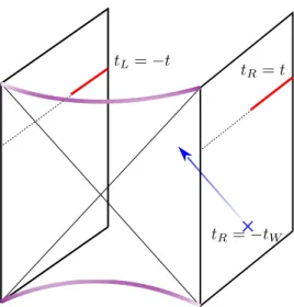
Figure 1. We consider a setup in which the eternal black hole is perturbed by an operator insertion at early times (blue cross). We calculate the relative entropy of the subsystem drawn with red between the TFD state and its perturbation.

The AdS/CFT correspondence [34] gives an excellent tool to analytically study quantum chaos in strongly coupled systems. A particularly useful setup is the Shenker Stanford process [35], in which one perturbs a thermofield double (TFD) state, which is holograph- ically dual to a two sided eternal black hole, by injecting energy on one side. In the dual gravity picture this amounts to sending a shock wave into the black hole. This process was argued to be chaotic, in particular, time evolution of the mutual information was calculated in [35]. In the present paper, we will be concerned with the relative entropy between the TFD state and its perturbation with the shockwave, both in the case of translational invariant and localized shocks. We take the spatial subsystem to be the union of the half line on both boundaries, see figure 1.

We will calculate this relative entropy in a holographic two dimensional conformal field theory (CFT) with large central charge and show that it indeed diagnoses scrambling. The result is that the relative entropy is initially proportional to the central charge of the CFT, but it decays exponentially in time. Assuming that the subsystem is large enough,⁶ there are two different exponential behaviours. Initially, the decay goes as exp(−^2π_β t) until times β t ∼βlogE, where E is roughly the total energy of the perturbation. In our setup, this energy will be large, but orderc⁰ in terms of the central charge c. We will argue that this decay rate is universal as it comes from the modular Hamiltonian piece. After this, the decay crosses over to exp(−^4π_β t). We will argue that in a generic CFT, the rate of this second decay is related to the behavior of out of time order (OTO) correlators in the Lyapunov regime, so that it is sensitive to chaos. This argument comes from doing the calculation using the replica trick combined with largecvacuum block techniques [36], besides directly

6When the subsystem is smaller than the scrambling time, its size gives the relevant timescale when the relative entropy drops to order one.

(7)

JHEP07(2018)002

applying the Ryu-Takayanagi formula [37]. We will see that Lyapunov regime shows up in the replica correlators. This second decay continues until the relative entropy becomes of order one at the scrambling timet∼βlogc, at which point quantum corrections to the Ryu- Takayanagi formula start to matter and we can no longer trust the result. We note that the exponential decay in time is something new compared to the typical linear or logarithmic time dependence of the entanglement entropy or the mutual information [38–42].

Another interesting feature is the dependence on the time when the shockwave is inserted. The sooner the shockwave is inserted, the larger the perturbation to the TFD state is on the t = 0 slice. In fact, a shockwave entering at time t =−t_W results in a relative entropy proportional toe^2π^β^t^W.⁷ This quantifies how far we end up with from the TFD state as a result of such an earlier perturbation, which has a similar flavour as the butterfly effect.

We will argue however that this kind of dependence is universal in conformal field theories, so it is not directly related to the Lyapunov exponent. It would be very interesting though if this universal growth could be used to understand the chaos bound of [4] from an information theoretic point of view. We will show that this relative entropy bounds out of time order correlators, though unfortunately we were not able to relate to their rate of change.

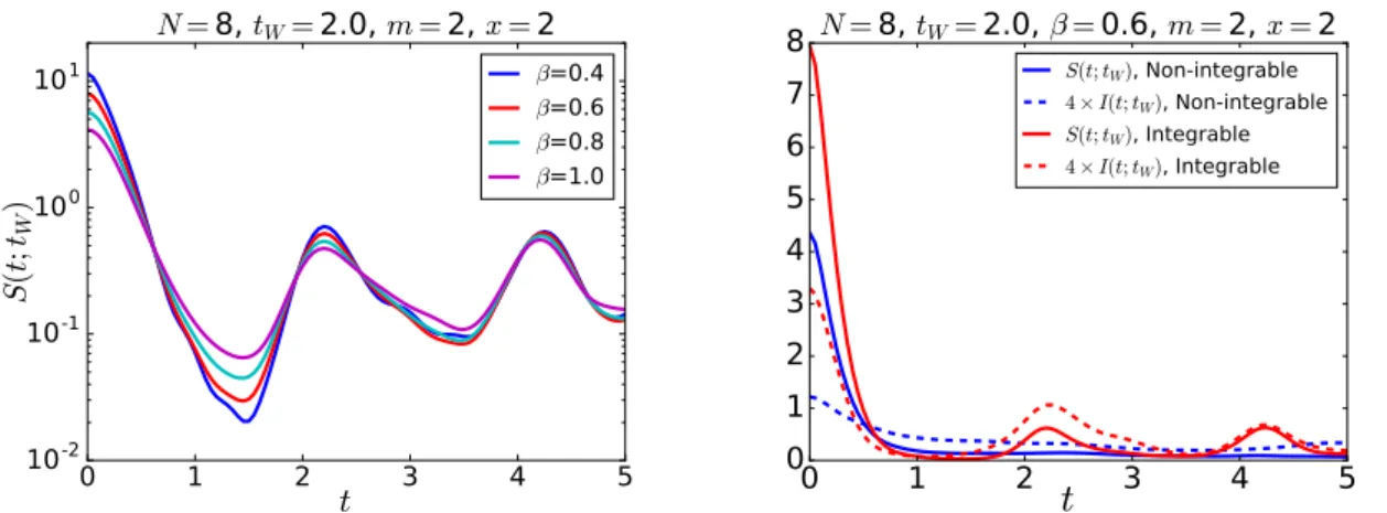
In addition to the holographic results, we perform numerical calculation of this relative entropy in a spin chain model. The main observation is that after the decay in t stops, the relative entropy stays small for a chaotic system, while has revivals comparable with the initial value for integrable systems.⁸ In this regard, it behaves similarly to the mutual information or the tripartite information. In addition to this, we will observe that the early time decay is exponential both for the chaotic and integrable cases. The exponent is proportional to the temperature similarly to the CFT case.

The organization of this paper is as follows. In section 2, we explain our setup in the setting of two dimensional conformal field theories. We show using the replica trick that the relative entropy is determined by how the replica correlators analytically continue in the replica index in their Regge-limit. Then, we obtain a concrete formula by approximating these correlators with the largecvacuum Virasoro block. We spend section3explaining the features of this formula and making some comments about the expected time dependence for non-holographic large c theories via a possible connection to the Maldacena-Shenker- Stanford (MSS) chaos bound. Sections 4 and 5are devoted to calculations of the relative entropy using the Ryu-Takayanagi formula, for translationally invariant and local perturbations respectively. In section6we present our numerical results for the spin chain model.

We have appendixA complementing some calculations in section 2. In appendixBwe de- scribe a generalization of our relative entropy to the case when both states are deformations of the thermofield double, while in appendix Cwe generalize the holographic calculations of section4 to the case when the subsystem has finite size.

7Note that the combined dependence ont, describing the location of the time slice, and tW describing the insertion of the shock is nontrivial, because the TFD state is not invariant under time translations.

8Similar revivals for single sided global quenches in rational CFTs were studied in [43]. Also, time evolutions in the process and its recurrence was studied in [44].

(8)

JHEP07(2018)002

2 Localized perturbations

In this section, we explain our setup in the CFT, and how to calculate the relative entropy of interest using correlation functions. These correlation functions have several distinct OPE- like limits, depending on the causality relation between the subsystem and the local perturbations. The discussion of this is very much similar to those found in [41,42], where the time evolution of entanglement entropy for local quenches on thermal backgrounds were studied.

We will eventually focus on the relative entropy between a thermofield double state and its perturbations, where we know the exact expression of the modular Hamiltonian.

The relative entropy consists of the modular Hamiltonian part as well as the entanglement entropy part. We first explain the way to evaluate the modular Hamiltonian part with again paying attention to the causality of the set up.

The entanglement entropy part can be evaluated by a four point function involving twist operators in the cyclic orbifold of the original CFT. In a CFT with a gravity dual, this four point function can be well approximated by the vacuum Virasoro conformal block and the result agrees with the holographic one given by the Ryu-Takayanagi formula. In the next section we will use the four point function expression to discuss a possible connection between the time dependence of the relative entropy and the MSS chaos bound [4].

2.1 General replica setup

We will consider a two dimensional conformal field theory (CFT) and the thermofield double state

|T F Di= 1

√ Z

X

n

e^−βEⁿ^/2|ni_L|ni_R∈CF T_L⊗CF T_R. (2.1) One can create this state by cutting up in half the Euclidean path integral on the cylinder which calculates the thermal partition function. The two lines of the cut correspond to the left and the right copy of the CFT. When the CFT has a gravitational dual, the |T F Di state is dual to the two-sided AdS-Schwarzschild black hole, connecting the two boundaries.

The |T F Di state is a special model of a non-equilibrium quench state with respect to the time evolution generated by H_L+H_R, whereH is the Hamiltonian of the single CFT [40].

We will be interested in local perturbations of the |T F Di state

V(x, tp−i)|T F Di, W(x, tp−i)|T F Di, (2.2) whereV andW are local primary operators of the CFT. The role of the Euclidean time shift is to regulate the energy of these states and to make them normalizable. We will reduce these states to a subsystem which consists of a half line on both CFTs. The reduced density matrix is calculated as a path integral on the cylinder of circumference β with cuts corre- sponding to the in and out indices of the matrix, see figure 2. The cuts are running from

P_R¹ : (x, t_E) = (0, it) to P_R^∞: (x, t_E) = (∞, it) (2.3) and from

P_L¹ : (x, t_E) = (0,−it+β/2) to P_L^∞(x, t_E) = (∞,−it+β/2), (2.4)

(9)

JHEP07(2018)002

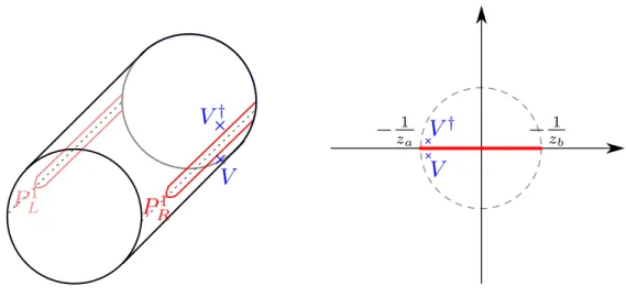
Figure 2. Euclidean path integral creating the perturbed state. Left: drawn on the cylinder, red line is the cut along the subsystem, blue crosses are operator insertions. Right: drawn when mapped to the plane. Red line is the cut, blue crosses are operator insertions. Note that we have applied a global conformal mapz7→ −1/z on the figure compared to the text to make the location of the cut more illustrative.

and operator insertions

V at (w₁,w¯₁) = (x−t_p+i, x+t_p−i) and V^† at (w₂,w¯₂) = (x−t_p−i, x+t_p+i), (2.5) where w = x+itE, ¯w = x−itE. When mapped to the plane with the map z = e^2π^β^w, we can see that the two points P_R^∞ and P_L^∞ are secretly the same and we get a single cut running from

(za=e⁻^2π^β ^t,z¯a=e^2π^β ^t) to (z_b =−e^2π^β^t,z¯_b =−e⁻^2π^β ^t), (2.6) and operator insertions at

V : z1 =z∗e⁻ⁱ^2π^β, z¯1 = ¯z∗eⁱ^2π^β, V^†: z₂ =z∗eⁱ^2π^β, z¯₂ = ¯z∗e⁻ⁱ^2π^β ,

(2.7) wherez∗ =e^2π^β^(x−t^p⁾, ¯z∗=e^2π^β^(x+t^p⁾.

We will use the replica trick of [45] for the relative entropy S(ρ_V||ρ_W) =−lim

n→1∂_nlog Trρⁿ_V

TrρVρⁿ⁻¹_W . (2.8)

We now want to compute Trρⁿ_V and Trρ_Vρⁿ⁻¹_W , which are given by the Euclidean path integral on ann-sheeted cylinder with appropriate operator insertions on each sheet. We do this by uniformizing to the plane with the map ˜z=

z−e⁻^2π^β^t z+e

2π β t

1/n

and ¯z˜=

z−e¯ ^2π^β^t

¯ z+e⁻

2π βt

1/n

. We get the following insertion positions

z_1,2;k=e^2πikⁿ e⁻^βn^2π^t





sinh^π(w^1,2_β^+t) cosh^π(w^1,2_β ^−t)





1 n

, z¯_1,2;k=e⁻^2πikⁿ e^βn^2π^t





sinh^{π( ¯}^w^1,2_β ^−t) cosh^{π( ¯}^w^1,2_β ^+t)





1 n

. (2.9)

(10)

JHEP07(2018)002

We have dropped the tilde from these insertion points, to ease the notation. It should be understood that a coordinate with a subscript k means that the coordinate is on the uniformized plane. The quantities of interest are then computed by the following correlation functions on the plane

Trρⁿ_V

Trρⁿ_{T F D} = hQn

k=1V(z1;k,z¯1;k)V^†(z2;k,z¯2;k)i Qn

k=1hV(z_1;k,z¯_1;k)V^†(z_2;k,z¯_2;k)i, TrρVρⁿ⁻¹_W

Trρⁿ_{T F D} = hV(z_1;1,z¯_1;1)V^†(z_2;1,z¯_2;1)Q_n

k=2W(z_1;k,z¯_1;k)W^†(z_2;k,z¯_2;k)i hV(z1;1,z¯1;1)V^†(z2;1,z¯2;1)iQn

k=2hW(z1;k,z¯1;k)W^†(z2;k,z¯2;k)i.

(2.10)

Here,ρT F D is the density matrix for the TFD state, without operator insertions.

2.1.1 Small limits

The insertion points (2.7) approach each other in a particular way when we take → 0.

The physically distinct cases are controlled by the signs of ζ1,2= Re





sinh^π(w^1,2_β^+t) cosh^π(w^1,2_β^−t)



, ζ¯1,2 = Re





sinh^{π( ¯}^w^1,2_β ^−t) cosh^{π( ¯}^w^1,2_β ^+t)



, (2.11)

because when the argument of the nth root in (2.9) is negative, the insertion point picks up an extra factor of e^±i^πⁿ, where the sign depends on the sign of the i shift in (2.7).

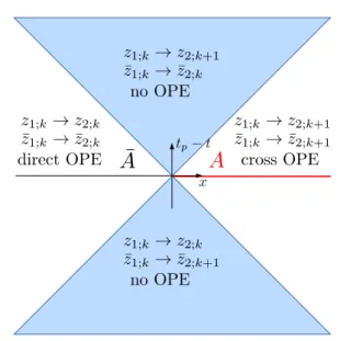
This difference corresponds to crossing the cut once. The signs of ζ1,2,ζ¯1,2 are controlled by the causal relationship between the operator insertion point and the endpoint of the subsystem, see figure3. There are the following cases.

• When|x|>|t−tp|, we have either bothζ1,2 >0 and ¯ζ1,2>0 (whenx > tp−t >−x), so the argument of the nth root is positive, or both ζ_1,2 < 0 and ¯ζ_1,2 < 0 (when x < tp−t < −x), so the argument of the root is negative. In the x > tp−t > −x case we have an OPE limit as →0

z1;k→z2;k z¯1;k →z¯2;k. (2.12) This situation is analogous to a small subsystem limit in the setup of globally excited states considered in [46,47], with roughlyplaying the role of the size of the subsystem. It follows that the relative entropy vanishes as→0. Physically, this is because the local operator insertion is in the causal domain of dependence of thetraced out region. Therefore, the RDMs of states with such insertions are the same and we expect the relative entropy to indeed vanish as → 0. This situation is tractable entirely with the OPE, we give a summary of how the relative entropy behaves in appendixA.

In the case x < t_p−t <−x, half of the operators actually cross the cut once more and we have

z_1;k→z_2;k+1 z¯_1;k →z¯_2;k+1. (2.13)

This situation is analogous to a large subsystem size limit for globally excited states, therefore the relative entropy must diverge as→0 (this is because we are comparing

(11)

JHEP07(2018)002

pure states in this limit). Physically, this is when the insertion point is in the causal domain of dependence of the region that we are not tracing over, so it is natural that the relative entropy does not vanish as → 0. We mention here, that for the correlators (2.10), which compute the replica relative entropy, this limit is still an OPE limit and we can calculate their expansion in . However, we cannot take the analytic continuation because of a singularity in the complex plane that moves to the point that we are expanding around (= 0 in the present context) when n→1.

This is a feature of correlation functions that break replica symmetry. It is presently unclear to us if there is a way around this obstacle.

• In the other case, when |x|<|t−tp|, i.e. the insertion is in causal contact with the endpoint of the subsystem, we have either

ζ1,2 <0, ζ¯1,2 >0, when tp−t >|x|, (2.14) or

ζ1,2 >0, ζ¯1,2 <0, when tp−t <−|x|. (2.15) This is a weird situation, as the different chiralities of the operator insertions appear to be on different sheets as →0. In the first case we have

z_1,k →z_2,k+1

¯

z_1,k →z¯_2,k, (2.16)

while in the second case we have

z_1,k→z_2,k

¯

z_1,k→z¯_2,k+1. (2.17)

This is not an OPE limit, instead it is a very similar limit as the one considered in [48] in the context of entanglement scrambling. In the case of the replica symmetry preserving correlation function, we will soon see that this corresponds to a Regge limit in the cyclic orbifold theory.

We summarize the above cases on figure 3.

2.1.2 Chaos and the late time limit

Here we argue that in the case when|x|<|t−t_p|, i.e. the operator insertion is in the future or past lightcone of the endpoint of the subsystem, the replica relative entropy is sensitive to the integrability of the CFT. Consider for example the case tp−t <−|x|, when we have z_1,k → z_2,k and ¯z_1,k →z¯_2,k+1. The point is that the way these coordinates approach each other has a hierarchy. Forx= 0 one has

z_1,k−z_2,k

¯

z1,k−¯z2,k+1

=e⁻^βn^4π^t. (2.18)

(12)

JHEP07(2018)002

Figure 3. Regions of the operator insertion (x, tp) relative to the endpoint of the subsystem (0, t) on the right CFT, and the respective →0 limit of the positions of the operator insertions on the replica manifold.

We see that for t large enough, this is small and we are effectively first takingz_1,k → z_2,k and then ¯z_1,k → z¯_2,k+1.⁹ The effect of first taking z_1,k → z_2,k is to project to chiral operatorsh= 0 in the V ×V^†OPE channels of the correlators (2.10). This means that in this limit the entire correlator is fixed by the chiral algebra of the CFT, so it is linked to the amount of symmetries that the CFT has. This is very similar to the way the depth of the quasiparticle dip works in the two interval entanglement entropy of a quench state [48].

2.2 The modular Hamiltonian part

After the general discussion of the previous section, we are now going to restrict to the case when one of the states is the unperturbed thermofield double.¹⁰ In this case, we can calculate the relative entropy as

S(ρW||ρ_{T F D}) =hW|K_{T F D}|Wi −

S(ρW)−S(ρT F D)

, S(ρ)≡ −Trρlogρ, (2.19) where K_{T F D} = −logρ_{T F D} +α is the modular Hamiltonian for the thermofield double state where we have fixed the number α so thathT F D|K_{T F D}|T F Di = 0. In the present subsection we evaluatehW|K_{T F D}|Wi, which is entirely fixed by kinematics.

In this section, we will consider the slightly generalized subsystem consisting of the union of the intervals

A: (t, x > L) and B : (−t−iβ/2, x >0), (2.20)

9Fortp−t >|x|, we can get such a hierarchy fortlargely negative, in that case we first take ¯z1,k→z¯2,k

and thenz1,k→z2,k+1.

10We will further discuss the relative entropy between two perturbed states in appendixB.

(13)

JHEP07(2018)002

i.e. a half line with adjustable end pointLon right CFT and a half line on left CFT. This is still effectively a single interval setup and in terms of light cone coordinates the endpoints are

(y₁,y¯₁) = (L−t, L+t) and (y₂,y¯₂) = (t+iβ/2,−t−iβ/2). (2.21) The left moving part of the modular Hamiltonian can be obtained by the conformal map z=e^2π^β ^y from the vacuum modular Hamiltonian on the plane

Kz1,z2 = Z z2

z1

(z2−z)(z−z1) z2−z1

T(z)dz (2.22)

along the lines of [49]. It is given by K_L= β

π Z

C

dycoshπ^y−t_β sinhπ^t+y−L_β

coshπ^L−2t_β T(y), (2.23)

where the contour C runs from y₁ = L−t along the line Imy = 0 to y = ∞, where it turns up to y = ∞+iβ/2 and runs back to y2 = iβ/2, see the left of figure 4. This is just an integral along the subsystem shown on figure2. The right moving part is obtained by complex conjugation of this contour, and a replacement t→ −t in both the endpoint positions and the integrand. The complete modular Hamiltonian is

K=−K_L−KR, (2.24)

becauseT00=−_2π¹ (T+ ¯T). The stress tensor expectation valuehΨ|T(y)|Ψi in the state of interest (2.7) is computed from the three point function,

hW(w₁)T(y)W(w₂)i hW(w1)W(w2)i =

h_W

β

πsinhπ^w¹^−w_β ²2

β

π sinhπ^w¹_β^−y2

β

πsinhπ^y−w_β ²2, (2.25) here we employed the normalization ofW,hW(∞)W(0)i=1. In our set upw₁, w₂are given by

w₁=x−t_p+i, w₂=x−t_p−i, (2.26) With the aid of this, we can write the explicit expression for the expectation value hK_Li ≡ hW|K_L|Wi of (2.23)

hK_Li= 4πhW

β sin²2π β

Z

C

dycoshπ^y−t_β sinhπ^t+y−L_β coshπ^L−2t_β

−1

cos^2π_β −cosh^2π_β(y−a)

2, (2.27) witha=x−t_pfor the present left moving case, while the right moving case is obtained again by complex conjugation andt→ −t, t_p→ −t_p. The integrand has poles aty=a±i+iβk, k∈Z. We have two possible cases:

• In case L−t > a =x−tp the contour stays clear of the vicinity of any poles. We may send cos^2π_β → 1 in the integrand and we can deform the contour into the sum of two finite straight pieces, each of which on the integrand stays finite. The result in this case is clearly finite, therefore we have hKi ∼² coming from the prefactor of the integral.

(14)

JHEP07(2018)002

Figure 4. Left: the modular Hamiltonian contour in (2.27). Right: the deformed contour when a > L−t. Whena < L−t, the contour stays clear of the poles ata±iand we can deform it into a finite length one without picking up any residue.

• When L−t < a=x−t_p, we can deform the contour through the pole at y=a+i to obtain again a finite length contour which stays clear of singularities as → 0, see the right of figure 4. The price we pay for this is that we pick up a residue at y=a+i. Therefore, in this case we have

hK_Li= 4πh_W β

(

 β 2

sinh^π(L−2t)_β −sinh^π(2a−L)_β

sin^2π_β cosh^π(L−2t)_β +O()





+ sin² 2π β

finite

) .

(2.28)

Notice that the conditionL−t < aguarantees this to be negative. Note that the left moving part of the total energy of the state can be obtained by takingt→ ∞in this formula, and it isE_W ∼h_W/sin^2π_β . To obtain the right moving part of the modular Hamiltonian expectation value hK_Ri, we set t→ −t, t_p → −t_p (the results are obvi- ously real), and we needt+L <¯a=x+tp to obtain a nonvanishing result as→0.

We will now restrict again to the symmetric interval caseL= 0. We have seen that the left moving part contributes only when−t < x−tp while the right moving part contributes only when t < x+t_p. These two cases correspond to the union of the right and bottom wedges for the case −t < x−t_p and the union of the right and top wedges for t < x+t_p on figure3. There are the following cases.

• Top. The perturbing operator W is inserted in the causal future of the endpoint of the subsystem. We see that only the right moving part contributes to nonvanishing pieces in. The total modular Hamiltonian contribution is

hKi=−hK_Ri= 2h_Wπsinh^2π(x+t_β ^p⁾ −sinh^2πt_β

sin^2π_β cosh^2πt_β . (2.29) We have t < x+t_p in this region ensuring positivity.

(15)

JHEP07(2018)002

• Bottom. The operator is inserted in the causal past of the endpoint of the subsystem.

In this case, only the left moving part contributed, giving hKi=−hK_Li= 2h_Wπsinh^2πt_β + sinh^2π(x−t_β ^p⁾

sin^2π_β cosh^2πt_β (2.30) Here, t > t_p −x ensures positivity. We will have in mind a situation when the perturbing operator is inserted at some early time t_p <0, |t_p| 1, while we follow the evolution int.

• Right. This is the causal diamond of the subsystem. In this case both the left and right moving parts contribute, giving in total

hKi=−hK_Li − hK_Ri

= 4h_Wπcosh^2πt_β^psinh^2πx_β

sin^2π_β cosh^2πt_β . (2.31) Here,x >0 ensures positivity.

• Left. This is the causal diamond of the complementary subsystem. In this case, neither the left nor the right moving part contributes and the result is

hKi ∼². (2.32)

We will not try to evaluate the finite integrals in this case, instead we give a separate treatment of the relative entropy in appendix A.

2.3 The entanglement entropy part in general

The entanglement entropy part in (2.19) in our two sided setup was studied before in [42].

Here we review this setup in a slightly different way which makes the connection to the behaviour of OTO correlators more transparent. To calculate the entanglement entropy in (2.19), we can use aZnsymmetric replica trick, which can be implemented in the orbifold theoryCF Tⁿ/Zn, see e.g. [50,51]. In this case, we can write

Trρⁿ_W

Trρⁿ_{T F D} = h˜σn(z_b,z¯_b)[W^†]^⊗n(z1,z¯1)σn(za,z¯a)W^⊗n(z2,z¯2)i

h˜σ_n(z_b,z¯_b)σ_n(z_a,z¯_a)ih[W^†]^⊗n(z₁,z¯₁)W^⊗n(z₂,z¯₂)i. (2.33) Here σn and ˜σn are the elementary Zn twist and anti-twist, and the expectation value is in the theory CF Tⁿ/Zn. The operator ordering in the nominator reflects the Euclidean cylinder time order for the operators: W andW^† has∓,σ_n has 0 and ˜σ_n hasβ/2.

We can use a global conformal map to map these operators to ∞,1, u,0. There is no Jacobian factor coming from this, because it is cancelled by the two-point function factors in the denominator. The cross-ratio is

u= (z1−z2)(zb−za) (z2−za)(z1−z_b)

= isin(^2π_β ) cosh(^2π_βt)

sinh^π_β(t−tp+x+i) cosh^π_β(t+tp−x+i),

(2.34)