Convergence of public and private enterprise wages in a transition economy: Evidence from a distributional decomposition in Vietnam, 2002 2014
著者(英) Tien Manh Vu, Hiroyuki Yamada journal or
publication title
AGI Working Paper Series
volume 2017‑10
page range 1‑25
year 2017‑04
URL http://id.nii.ac.jp/1270/00000130/
Convergence of public and private enterprise wages in a transition economy: Evidence from a distributional
decomposition in Vietnam, 2002–2014
Tien Manh Vu
Asian Growth Research Institute and Osaka University
Hiroyuki Yamada
Faculty of Economics, Keio University
Working Paper Series Vol. 2017-10 April 2017
The views expressed in this publication are those of the author(s) and do not necessarily reflect those of the Institute.
No part of this article may be used reproduced in any manner whatsoever without written permission except in the case of brief quotations embodied in articles and reviews. For information, please write to the Institute.
Asian Growth Research Institute
Convergence of public and private enterprise wages in a transition economy: Evidence from a distributional decomposition in Vietnam, 2002–2014
1Tien Manh Vu
2Asian Growth Research Institute and Osaka University Hiroyuki Yamada
Faculty of Economics, Keio University Abstract
We examine the transition of state-owned enterprises (SOEs) in Vietnam from a wage perspective by decomposing the difference in wage distributions between SOE employees and non-SOE employees during the period 2002–2014. In 2002, SOE employees enjoyed higher pay than non-SOE employees owing to characteristics difference and any factors other than either the price of skills or the characteristics difference, so-called residuals difference.
University graduates were the main contributor to the endowments difference. However, we found that SOE pay schemes converged with those of non-SOEs by 2014, in terms of both the price of skills and residuals.
Keywords: Wage, wage decomposition, wage distribution, state-owned enterprises, transition, Vietnam
JEL classifications: J30, J45, O15, P31
1
Acknowledgements: This work was supported by JSPS (Japan Society for the Promotion of Science) KAKENHI Grant Number 15H01950, a project grant from the Asian Growth Research Institute, and a grant from the MEXT Joint Usage/Research Center at the Institute of Social and Economic Research, Osaka University.
2
Corresponding author. Contact: 11–4 Otemachi, Kokura-kita, Kitakyushu, Fukuoka 803–0814, JAPAN
Tel.: +81–93–583–6202, Fax: +81–93–583–6576. E–mail: [email protected]
1. Introduction
For many decades, Vietnamese state-owned enterprises (SOEs) have been given top priority in terms of resource allocations in all state plans, with the aim that they would be the leading sector of the whole economy. However, both macroeconomic and microeconomic data (household and firm surveys) show that SOEs are reducing their employment shares in the Vietnamese economy. Similar to Fukase (2014) that used the Vietnamese Enterprises Survey Data for 2000–2007 and General Statistics Office (GSO) (2017a) aggregate data, our own calculations show that the share of the private sector including both domestic private firms and foreign affiliated firms was higher than that of the SOEs by 2005, as in Figure 1. In 2014, the private sector was the dominant employer providing paid jobs in Vietnam.
[Insert Figure 1 here]
Human capital development and productivity improvements are important to the survival and development of firms, and the growth of the private sector has led to increasing demand for highly-productive employees. Thus, offering competitive wages and wage-related benefits to attract productive employees has become important for the private sector and, perhaps, SOEs.
Therefore, the purpose of this study is to examine the transition of SOEs from a wage perspective by decomposing the wage gap distribution between SOE employees and other employees that offered formal employment. Our study makes some major contributions to the existing literature. First, it is one of few studies that consider differences along the wage distribution, rather than making the (strong) assumption that the difference is constant. Second, as discussed in detail below, our analysis decomposes the difference in the wage distribution into three separate components: the differences in the coefficients, the characteristics (endowments), and the residuals (interactions). Third, we are able not only to test for the significance of each decomposed component over time, but also to estimate the contribution of each covariate to each decomposed component. Our analysis provides new insights into the attractiveness of each sector to workers.
We use data from 2002 to 2014 from the Vietnamese Household Living Standard
Survey (VHLSS) at four-year intervals. We focus on a formal employment threshold by
selecting individuals who had only a job, and who were not students, government officers, or
self-employed and did not work for other households. We apply methods suggested by
Chernozhukov, Fernandez-Val, and Melly (2013) and a recentered influence function
regression by Firpo, Fortin, and Lemieux (2009) to decompose the wage distribution between SOE employees and non-SOE employees.
We obtain important evidence of wage convergence between SOE employees and non- SOE employees. During the period 2002–2014, the price of skills in the two sectors converged.
We find that the main difference in the wage distribution was the result of the differences in the distributions of skills and residuals during 2002–2010. The concentration of university graduates in SOEs was the main contributor to the endowments difference. However, we observe a gradual change and another important convergence in 2014: the residuals difference is vanishing at this point.
This study is organized as follows. The next section discusses the relevant literature on SOEs in transition economies and wage differences between public and private sectors particularly in Vietnam. Section 3 presents the data and how we select the samples. Section 4 provides the econometrics method and the model specification which could provide new insights to the difference. In Section 5, we report the results. In Section 6, we summarize and discuss some implications for policy and research agendas.
2. Related literature
2.1 Changes in SOEs and non-SOEs
In general, political will plays an important part in determining wages in the public sector, whereas the market environment has the leading role in the private sector (Gregory and Borland, 1999). However, whether SOEs in transition economies is one of the cases is not easy to identify.
Privatization among SOEs occurs in various ways in transition economies. Shi and Sun
(2016) noted that privatization could occur through a voucher mechanism, such as the almost
free share transfer to workers in Russia, or through cash auctions combined with public
subscription, as occurred in Lithuania. SOE privatization in China commenced with the
philosophy of ‘keep the large, privatize the small’ (Shi and Sun, 2016). From a political
economy perspective, Brezis and Schnytzer (2003) argued that privatization methods can be
classified into two types: ‘embezzlement’ (which applies to the practices of the East European
countries) and ‘Market-Leninism’ (the method applied in China and Vietnam). The difference
between the two methods is that, under the latter, certain (often higher) shares are retained by
the state, which enables it to maintain control. Thus, the autonomy of SOE managers might
vary because the state retains a different portion of shares in certain SOEs, especially in the case of China and Vietnam, giving it varying degrees of control.
The number of Vietnamese SOEs is falling sharply, and some of those remaining are providing offers for outsiders to buy its shares. The number of SOEs fell from 12,000 to approximately 6,000 over the period 1990–1994 (Painter, 2005). Painter (2005) suggested that Vietnamese SOE directors won greater autonomy after state subsidies were reduced or eliminated over the period 1986–1992. However, by 2004, 2,242 SOEs were equitized but the state still held 38.1 percent of the total shares. The proportion of shares owned by the state was higher than in Georgia, Kazakhstan, Kyrgyz, Moldova, Russia, and the Ukraine in 1997 (Loc, Lanjouw, and Lensink, 2006). This gradual transition allowed outsiders to buy shares without the state losing control of the SOEs (Brezis and Schnytzer, 2003).
Meanwhile, Vietnamese workers have a greater chance of finding jobs outside SOEs as a result of the growth of the private sector. Painter (2005) noted that by the end of 2002, there were about 56,000 newly established firms regulated under the first Laws on Enterprises in Vietnam. Besides, as seen in Figure 1, the employment share of the private sector was the largest by 2014 while that of SOEs reduced sharply. The free trade accessions, including the US–Vietnam Bilateral Trade Agreement in 2001 and Vietnam’s membership in the World Trade Organization in 2007, created more paid (formal) jobs and even the possibility of higher pay in the private sector. Vu and Yamada (2017) calculated that the proportion of ‘formal’
female (male) wage earners (working for either SOEs or non-SOEs) among the non-student, female (male) population was 5.8 (7.4) percent in 2002, but rose to 10.69 (11) percent in 2014.
Since the number of SOEs (non-SOEs) was reducing (increasing), the growth in formal employment would be mainly among non-SOEs. Ramstetter and Ngoc (2007) reported that foreign firms paid a higher wage premium than did SOEs in Vietnam during 2002–2006. All these facts raise questions about the wage equality between SOEs and non-SOEs in Vietnam.
In addition, differences in the regulations for SOEs and non-SOEs are declining in Vietnam. The first Laws on Enterprises became effective in 2000 and, in 2005, the updated Laws on Enterprises 2005
3omitted the different rules based on the ownership of firms.
However, other discrimination from a legal perspective continued. For example, Vu and Yamada (2017) noted that, until 2011, the regulations on minimum wages were treated differently between public sector and private sector, resulting in different minimum wage
3
Following that change, a further amendment was made to the Laws on Enterprises in 2015.
levels. Interestingly, the minimum wage for the private sector was higher than that for the public sector
4.
2.2 The public–private wage gap in Vietnam prior to accession to the World Trade Organization in 2007
Most of the previous studies on the public–private wage gap in Vietnam focus on the 1990s, when private-sector wage earners were not as prevalent as they became from the late 2000s and especially from the early 2010s. We find that there are many research gaps to be covered, given this changing context.
Based on analysis of the VHLSS for 1997–1998, Liu (2004) suggested that the private wage sector was underdeveloped and that wages were higher in the state sector. Defining the government sector and SOEs as the public (state) sector, Liu (2004) suggested that there were more females in the public sector than in the private sector. However, we note that including the government sector in the definition of the public sector means that, for 1997/98, 650,000 teachers with direct teaching duties in the general education sector are included in the calculation (by 2014, there were 850,000 such teachers) (GSO, 2017b). Over 70 percent of these teachers were females (GSO, 2017c). Thus, an alternative definition is required to compare SOEs and non-SOEs, especially in the new context, as shown in Figure 1.
Comparing the situations in 1993 and 2006, Imbert (2013) suggested that the wage gap between public employees and other employees was widening because the public sector selected the best workers. Imbert (2013) also implied that public-sector employees were underpaid during the 1990s, but that wages subsequently began to equalize with those of private employees. The question of why the best workers preferred to join or remain with the SOEs, given that they were often underpaid, or at best equally paid, has not been fully explained.
Imbert (2013) shared the view of Liu (2004) that women were better off in the public sector.
Meanwhile, evidence from the Vietnam Enterprises Survey, presented by Fukase (2014), and our calculation in Figure 1, show more women have continued to join the private sector and, from 2007, there were more women concentrated in the private sector, especially in foreign affiliated firms.
4
For example, government decree 03/2006/ND-CP set the minimum wage for the foreign sector at VND 870,000
in March 2006. The minimum for other sectors was VND 350,000. In 2008, dedicated to Region 4 (detailed region
classification can be found in the corresponding decree), government decree 111/2008/ND-CP set a minimum
wage of VND 950,000 for the foreign sector but its preceding decree 110/2008/ND-CP regulated VND 650,000
as the minimum wage for SOEs. In 2011, the minimum wage for the private sector in Region 4 was VND 1.4
million but for other sectors, it was VND 830,000.
Moreover, studies using the mean difference may not sufficiently capture the inequality in the new context. Vu and Yamada (2017) showed that the gender wage gap was not constant along the distributions in Vietnam during the period 2002–2014. The public and private enterprise wage gap distribution may not be an exception.
3. Data
We used the Vietnam Household Living Standard Survey (VHLSS) for 2002, 2006, 2010, and 2014, conducted by the General Statistics Office (GSO) of Vietnam. The two-stage stratified surveys have a country representative sample with a design similar to that of the Living Standard Measurement Study by the World Bank. The household sample sizes were 29,532 households (2002), 9,189 households (2006), 46,995 households (2010), and 9,399 households (2014). The surveys provide detailed information for each individual on personal characteristics (including age, gender, and education level) as well as information on paid work and wage premiums (including working hours, salary, and bonuses in cash and in kind).
We chose to focus on individuals who had a job, and who were not students, state officers, self-employed, or working for other households. We selected age thresholds from 15 to 55 years for both genders. A selection of up to 60 years of age would capture more informal female workers because the retirement age for women is 55 years and it is a very strict requirement in SOEs.
The wage calculation is the crucial issue. If salaries in cash are counted as the only contribution to the wage, any comparison between SOEs and non-SOEs would be biased because proportions of other related income than salaries differ. Thus, we counted any income related to the paid work in calculating the total earned wage. More specifically, the total earned wage equals the sum of salaries, bonuses for holidays, bonuses in cash and in kind, and any other income related to the paid job within the 12 months prior the survey. Similarly, we summed the total working hours in the same period for each individual. The total earned wage was converted to 2010 real prices using World Bank CPI
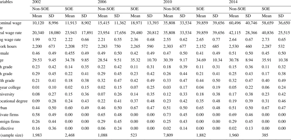
5and divided into the total working hours to construct the real wage rate. Then we transformed the real wage rate to logarithmic form. We trimmed 0.1 percent of respondents from each survey at both tails of the wage distribution prior to undertaking any analysis. The descriptive statistics are provided in Table 1.
5
Source: http://data.worldbank.org/indicator/FP.CPI.TOTL?end=2015&locations=VN&start=2000
[Insert Table 1 here]
The descriptive statistics show some interesting trends. As seen in Table 1, SOE employees had a higher average real wage than non-SOE employees in 2002 (about 17 percent higher). However, in 2014, they had a 3 percent lower average real wage than non-SOE employees. When the number of work hours is considered, the mean logarithm of the real wage rate difference between SOE employees and non-SOE employees gradually reduced over time;
it was 11.6 percent higher for SOE employees in 2002, fell to 6.8 percent higher in 2006, to 3.9 percent higher in 2010, and finally to only 3.4 percent higher in 2014. This is because although the average work hours of SOE employees was rather stable, those of non-SOE employees increased over time.
4. Methods
We apply two important methods in our analysis. The first method was suggested by Chernozhukov, Fernandez-Val, and Melly (2013) (hereafter referred to as CFM). The second method is a recentered influence function (RIF) regression, using the unconditional quantile regression by Firpo, Fortin, and Lemieux (2009). The key point of both methods is to estimate a counterfactual distribution of the first group of workers based on a component distributed as if it were the second group’s and the remaining components as if they were those of the first group.
4.1 The CFM method
The objective of the method is to estimate two important counterfactual distributions. The first is estimated from the characteristics distribution for the group of employees working for SOEs, the median (mean) coefficients from the group of employees working for SOEs, and the residual distribution from the group of employees working for non-SOEs. The second distribution is constructed from the characteristics distribution for the group of employees working for SOEs, and the conditional distribution of the skills of employees working for non- SOEs. Following the procedure suggested by Juhn, Murphy, and Pierce (1993), the total difference is decomposed into three components: coefficients, characteristics, and residuals.
.
(1)
More specifically, similarly to the procedure by Melly (2005), first, the method
estimates the counterfactual distribution of the wages, , , that would be
received by non-SOE employees if their skill distribution was similar to those of the SOE employees. are the estimated coefficients of non-SOE employees from a quantile regression by Koenker and Bassett (1978) and is the characteristics vector of employees in SOEs. The characteristics difference is the difference between , and , . The counterfactual wage distribution, if the median returns to skills for non-SOE employees were exactly the same as those of SOE employees, and if the residuals distribution were that of the non-SOE employees, is
,, . The
coefficients difference is the gap between
,, and
, . Thus, the detailed breakdown of (1)
6is:
, , ,
,
,
,, ,
, , . (2)
4.2 RIF regression and Oaxaca–Blinder decomposition
We apply the RIF regression suggested by Firpo, Fortin, and Lemieux (2009). In this specific case (using quantiles), the RIF regression can be called an unconditional quantile regression.
The recentered influence function, ; , is a sum of the influence function,
; , and the distributional statistic of interest, . is logarithm of the real wage rate. Then, the estimation results are used to decompose the contribution of each of the covariates using a procedure
7suggested by Oaxaca (1973) and Blinder (1973). More specifically, the difference in the logarithm of the real wage rate between the two groups at each quantile can be decomposed as follows:
∆ , , , ,
, and (3)
∆ , , , ,
,
. (4)
This can be simplified as follows:
6
A user-written Stata command, ‘cdeco_jmp’ by Chernozhukov, Fernandez-Val, and Melly eased our estimations.
The command can be found at https://sites.google.com/site/blaisemelly/computer-programs/inference-on-
counterfactual-distributions.7
As suggested by Firpo, Fortin, and Lemieux, we use another user-written Stata command, ‘oaxaca8’ by Jann
(2008) to decompose the results from the RIF regression. The detailed guideline from Firpo, Fortin, and Lemieux
for RIF regression and decompositions can be found at http://economics.ubc.ca/faculty-and-staff/nicole-fortin/.
. (5) Both methods, CFM and RIF regression, have advantages and disadvantages. One of the most important advantages of the first method is that it constructs simultaneous confidence sets, which help to test the functional hypotheses, including zero influence and constant influence. The test results help us to confirm whether the difference is minor or large and whether it is constant along the distribution or polarized. However, the CFM method cannot provide detail on the contribution of each covariate to the decomposed components. In contrast, the second method provides a possible linear decomposition of each of the covariates. Thus, by using the two methods, we are able to utilize the advantages of each method.
4.3 Specifications
We set the covariates as experience, based on age, and a set of educational dummies. Following the suggestion of Vu and Yamada (2017), we do not use projected experience, which is calculated as age minus years of schooling and minus seven years. We also use the squared age. The set of dummies for highest education obtained are, for school years completed, five years (primary school graduates), nine years (secondary school graduates), and 12 years (high school graduates), and, for post-school qualifications, three-year college graduates, four-year or more university graduates, and those with vocational degrees. This specification is the same in all data sets used. In the counterfactual distribution estimations, we set a 100-repetition bootstrap.
5. Results
5.1 The total wage gap and its decomposed components
The total wage gap between SOE employees and non-SOE employees was persistent. However, the coefficients differences were minor during the period 2002-2014 and the residuals differences diminished by 2014. We have four important pieces of evidence supporting these findings.
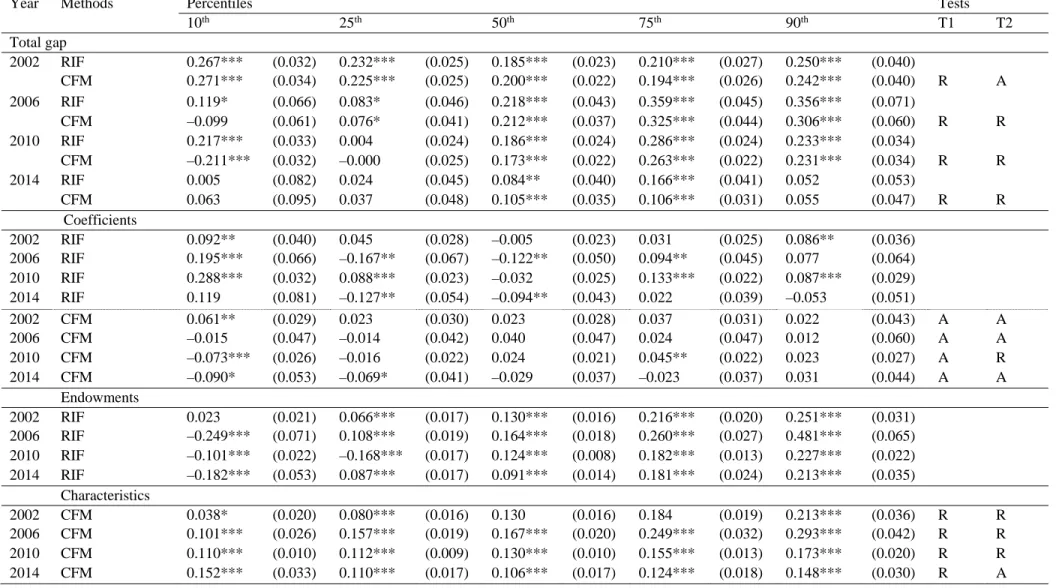
First, both methods showed that the total wage gap between SOE workers and non-
SOE workers was statistically significant, particularly for the middle and middle-to-high wage
distribution groups, as seen in Table 2. The tests for all quantile effects equal to zero were
rejected in all years (see columns T1 and T2 of Table 2). The persistent gap for the middle and
middle-to-high wage distribution groups is consistent with the findings of Turunen (2004) for
Russia. Turunen (2004) showed that white-collar workers for the state who held a university
degree and a managerial position were more likely to stay in the state sector. We note that the total difference is not constant along the income distribution. Except for 2002, all test results for the constant quantile effect in the CFM estimations (see column T2) support this argument (Figure 2 also illustrates this trend).
[Insert Table 2 here]
[Insert Figure 2 here]
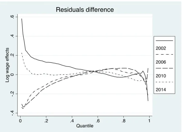
Second, we found that the coefficients difference was statistically insignificant in all selected waves. As shown in column T1 of Table 2, none of the test results for quantile effects different from zero were rejected. Third, the residuals difference disappeared in 2014 because the test for all corresponding quantile effects equaling zero was not rejected (see column T1 of Table 2). We will analyze this in detail in later in the paper.
[Insert Figures 3, 4, and 5 here]
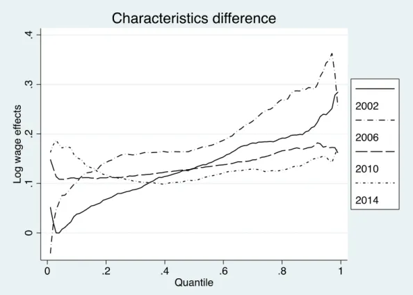
Fourth, the main contributor to the total difference was the characteristics (endowments) distribution difference. This is clear from both estimation methods. Tests for the zero quantile effect for the characteristics difference were all rejected, as seen in column T1 of Table 2.
However, the characteristics difference, which was higher at the right tail of the wage difference distribution (see Figure 5), returns to being flat and, finally, becomes constant along the distribution in 2014, as the tests in column T2 of Table 2 show.
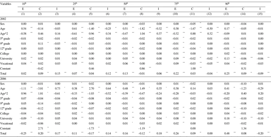
As the characteristics/endowments difference was the most important contributor to the total wage difference, we further break down the contribution of each characteristic using RIF regressions and the Oaxaca–Blinder decomposition.
5.2 University graduates and endowments difference
We found university graduates were the most important contributor to the endowments
difference between SOE employees and non-SOE employees. More specifically, in 2002,
university graduates were corresponding with increments of 57/38/40/52 percent
(0.04/0.05/0.09/0.13 log points) of the endowments difference at 25
th/50
th/75
th/90
thpercentiles,
as shown in columns 4, 7, 10, and 13 of Table 3. This suggests university graduates were more
available in SOEs at these percentiles of the endowments difference distribution in 2002. In
2006, they contributed 36/25/31/38 percent (0.04/0.04/0.08/0.18 log points) of the endowments
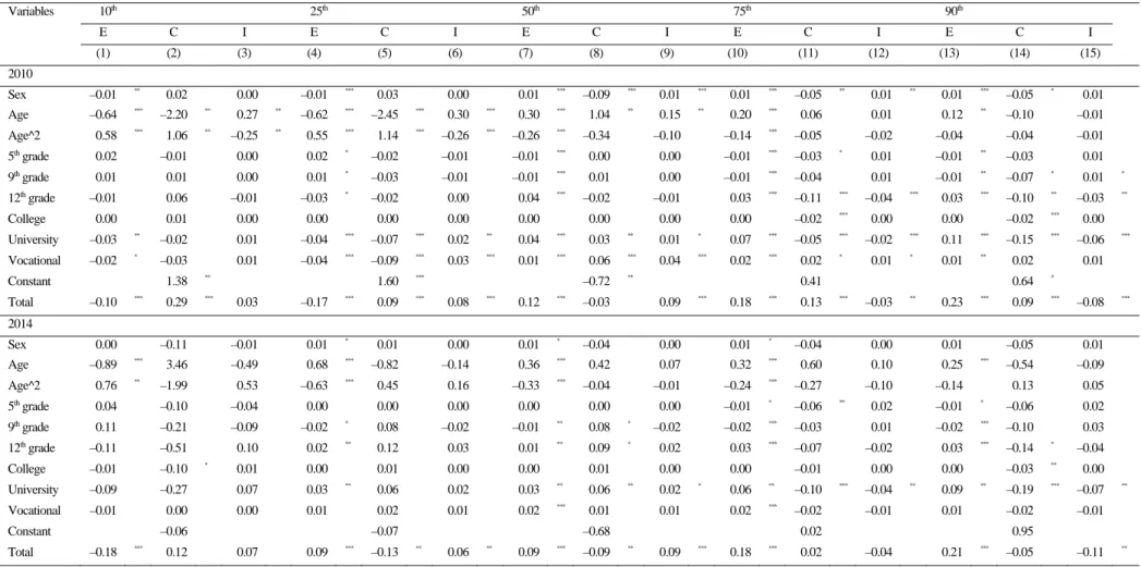
difference at the corresponding percentiles. In 2010, they were 33/38/48 percent
(0.04/0.07/0.11 log points) at 50
th, 75
th, 90
thpercentiles. In 2014, they returned to 33 percent
(0.03 log points) at 25
th/25
th/50
th/75
thpercentiles and 43 percent (0.09 log points) at 90
thpercentile.
[Insert Table 3 here]
However, during 2006-2014, at 10
thpercentile, university graduates were important contributor to reduce the endowments difference as the quantile effects are becoming negative (column 1 of Table 3). Within the scope of endowments difference, the negative coefficient of
“university” merely means SOE employees received lower income because they were less likely to have university degrees at this 10
thpercentile of the “income” distribution. It may be the case that non-SOEs were attractive and appeared more accessible to fresh university graduates commencing their career.
This result does not contradict the findings that university graduates in SOEs received lower returns to “university” in SOEs, which was found for the 75
thand 90
thpercentiles in 2002 (columns 11 and 12 of Table 3), the 90
thpercentile (column 14) in 2006, and at the 25
th, 75
th, and 90
thpercentiles (columns 5, 11, and 14) in 2010. We would argue that precedent regulations to lay off public employees based on education is the most likely explanation. Friedman (2004) indicated that, based on a survey conducted in 2000, Vietnamese SOE workers were in higher demand for formal training than were non-SOE workers. Thus, SOE workers may have sought to upgrade their educational qualifications so as to retain their positions when they were expecting the size of SOEs to contract. Over-concentration of university graduates may have occurred because, although employees were upgrading their educational qualifications, labor productivity may not have increased.
85.3 The convergence of pay schemes between SOEs and non-SOEs in 2014
We found that the pay schemes of SOEs converged with those of non-SOEs by 2014. First, the differences in coefficients were minimal in 2002, 2006, 2010, and 2014. Second, the residuals difference became statistically insignificant in 2014, as shown in column T1 of Table 2. Third, the characteristics differences were declining over time for the middle-to-high wage distribution groups as seen in Table 2. The remaining (positive) difference is the result of some component of the skills distribution. Except for 2010, when women were paid less in SOEs in terms of the average price of skills (see columns 8, 11, and 14 of Table 3), we found little evidence that women were paid differently by the price of skills in SOEs compared with non-
8
Friedman (2004) suggested that Vietnamese SOE workers even had lower labor productivity compared to non-
SOE workers.
SOEs in other years and percentiles. Our result differs from the results of Liu (2004), not only because of the time period difference but also because of the data selection.
Finally, we anticipate that the remaining difference between SOEs and non-SOEs will become increasingly smaller in the years to come. This is because there would be more options in the labor market for young and highly-educated workers with equivalent pay and because there would be little incentive for highly-educated workers to join SOEs, but more benefits from leaving SOEs. In 2014, the skill price was negative for most skill levels at the 75
thand 90
thpercentiles, for SOE employees (see columns 11 and 14 of Table 3). At the 50
thpercentile, the coefficients difference was negative despite some of the education level groups being paid more by SOEs. As a possible consequence, better-educated, highly-productive workers in these segments would be likely to leave the SOEs,
9which would lower the current endowment differences. However, we also acknowledge that those, who are relatively ‘old’ and self- selected to work for SOEs in the past, will remain. This is because they may have difficulty in matching their employable skills with the needs from non-SOEs at equivalent or higher wage rate.
6. Conclusions and discussion
In this paper, we have examined the transition of SOEs from a wage perspective, by decomposing the wage distribution difference between SOE and non-SOE employees during the period 2002–2014, using four Vietnamese household surveys of the same design and the same sample selection. Although SOE employees received higher pay in 2002 as a result of the characteristics difference and residuals, the coefficients difference was minimal along the wage distribution during 2002–2014. The characteristics difference fell over time at middle and middle-to-high wage distribution groups. University graduates were the main contributor to the endowments difference. However, by 2014, the residuals difference vanished and the pay schemes between SOEs and non-SOEs had converged.
The convergence of pay schemes between SOEs and non-SOEs has some implications for policy and research agendas. First, the Vietnamese government should keep treating SOEs as equivalent to non-SOEs from a legal perspective. Limiting the privileges applied to any sector creates a more competitive environment, increases wage equality among firms with different ownership structures, and results in more efficient resource allocations. Second,
9
The employees may stay if they have supervisory posts, as suggested by Turunen (2004). However, SOEs
cannot create enough such posts for all of these workers.
unless the state wishes to support inefficiency through public budgets/assets, more autonomy for SOE managers to restructure the current pay schemes is a must. Third, as SOEs pay as much as non-SOEs, a convergence in the characteristics difference is foreseeable. High productivity employees, if receiving lower pay, might leave the SOEs. However, rather than state policies attempting to prevent this, allowing it to happen will provide incentives for SOEs to restructure their pay schemes to become more attractive to high productivity employees. If SOEs can successfully change, the demand for expensive formal training that is not necessarily linked to higher productivity would disappear. In contrast, the demand for informal training and on-the-job training to improve productivity will rise. Finally, future studies of the public–
private enterprise wage gap in Vietnam should search for evidence of the disappearance of the characteristics differences. Once this has been found, any different settings to distinguish between SOEs and non-SOEs in wage-related estimations would become redundant.
References
Blinder, A. S. (1973). ‘Wage discrimination: Reduced form and structural estimates’, Journal of Human Resources, 8(4), pp. 436–455.
Brezis, E. S., and Schnytzer, A. (2003). ‘Why are the transition paths in China and Eastern Europe different? A political economy perspective’, Economics of Transition, 11(1), pp.
3–23.
Chernozhukov, V., Fernandez-Val, I., and Melly, B. (2013). ‘Inference on counterfactual distributions’, Econometrica, 81(6), pp. 2205–2268.
Firpo, S., Fortin, N. M., and Lemieux, T. (2009). ‘Unconditional quantile regressions’, Econometrica, 77(3), pp. 953–973.
Friedman, J. (2004). ‘Firm ownership and internal labour practices in a transition economy’, Economics of Transition, 12(2), pp. 333–366.
Fukase, E. (2014). ‘Foreign wage premium, gender and education: Insights from Vietnam household surveys’, The World Economy, 37(6), pp. 834–855.
Gregory, R. G. and Borland, J. (1999). ‘Recent developments in public sector labor markets’, in Ashenfelter, O. C., and Card, D. (ed.), Handbook of Labor Economics, Chapter 53 (Vol 3c, pp. 3573–3630), in the Netherlands: North Holland.
General Statistics Office of Vietnam. (2017a). Number of employees in enterprises as of December 31 by type of enterprise. Last accessed: February 10, 2017.
http://www.gso.gov.vn/Modules/Doc_Download.aspx?DocID=9771
General Statistics Office of Vietnam. (2017b). Number of teachers and pupils of general education as of 30 September. Last accessed: March 10, 2017.
http://www.gso.gov.vn/default_en.aspx?tabid=782
General Statistics Office of Vietnam. (2017c). Number of woman teachers and schoolgirls of general schools as of 30 September. Last accessed: March 10, 2017.
http://www.gso.gov.vn/default_en.aspx?tabid=782
Imbert, C. (2013). ‘Decomposing the labor market earnings inequality: the public and private sectors in Vietnam, 1993–2006’. The World Bank Economic Review, 27(1), pp. 55–79.
Jann, B. (2008). OAXACA8: Stata module to compute decompositions of outcome
differentials. URL: https://ideas.repec.org/c/boc/bocode/s450604.html. Last accessed:
December 24, 2016.
Juhn, C., Murphy, K. M., and Pierce, B. (1993). ‘Wage inequality and the rise in returns to skill’, Journal of Political Economy, 101(3), pp. 410–442.
Koenker, R. and Bassett, G. (1978). ‘Regression quantiles’, Econometrica, 46, pp. 33–50.
Liu, A. Y. C. (2004). ‘Sectoral gender wage gap in Vietnam’. Oxford Development Studies, 32(2), pp. 225–239.
Loc, T. D., Lanjouw, G., and Lensink, R. (2006). ‘The impact of privatization on firm performance in a transition economy. The case of Vietnam’, Economics of Transition, 14(2), pp. 349–389.
Melly, B. (2005). ‘Decomposition of differences in distribution using quantile regression’, Labour Economics, 12(4), pp. 577–590.
Oaxaca, R. (1973). ‘Male–female wage differentials in urban labor markets’, International Economic Review, 14(3), pp. 693–709.
Painter, M. (2005). ‘The politics of state sector reforms in Vietnam: contested agendas and uncertain trajectories’. Journal of Development Studies, 41(2), pp. 261–283.
Ramstetter, E. D. and Ngoc, P. M (2007). ‘Employee compensation, ownership, and producer concentration in Vietnam’s manufacturing industries’, AGI-Working Paper Series 2007–
07, Asian Growth Research Institute, Fukuoka, http://www.agi.or.jp/workingpapers/WP2007-07.pdf.
Shi, W., and Sun, J. (2016). ‘The impact of privatization on efficiency and profitability’,
Economics of Transition, 24(3), pp. 393–420.
Turunen, J. (2004). ‘Leaving state sector employment in Russia’, Economics of Transition, 12(1), pp. 129–152.
Vu, T. M. and Yamada, H. (2017). ‘Decomposing gender equality along the wage distribution
in Vietnam during the period 2002–14’, AGI-Working Paper Series 2017–03, Asian
Growth Research Institute, Fukuoka, http://www.agi.or.jp/workingpapers/WP2017-
04.pdf.
Table 1. Descriptive statistics
Variables 2002 2006 2010 2014
Non-SOE SOE Non-SOE SOE Non-SOE SOE Non-SOE SOE
Mean SD Mean SD Mean SD Mean SD Mean SD Mean SD Mean SD Mean SD Nominal wage
rate
10,120 8,996 11,913 8,902 15,415 11,362 18,971 13,393 35,808 33,534 39,859 39,656 60,496 40,746 58,659 36,650 Real wage rate 20,340 18,080 23,943 17,891 23,954 17,656 29,480 20,812 35,808 33,534 39,859 39,656 42,115 28,366 40,836 25,515 Log wage rate 1.99 0.72 2.22 0.66 2.21 0.55 2.36 0.68 2.55 0.62 2.65 0.77 2.64 0.67 2.73 0.65 Work hours 2,200 673 2,208 572 2,283 750 2,265 590 2,303 677 2,152 685 2,530 460 2,287 532 Female 0.46 0.49 0.455 0.49 0.49 0.50 0.42 0.49 0.47 0.50 0.41 0.49 0.51 0.50 0.45 0.50 Age 29.53 9.45 34.78 9.85 28.54 9.51 35.32 10.70 30.39 9.17 34.69 10.34 30.78 8.94 35.91 10.38 5th grade 0.23 0.42 0.14 0.35 0.22 0.42 0.11 0.31 0.18 0.39 0.11 0.31 0.15 0.36 0.11 0.32 9th grade 0.29 0.45 0.22 0.41 0.29 0.45 0.23 0.42 0.26 0.44 0.21 0.41 0.25 0.43 0.17 0.38 12th grade 0.21 0.41 0.18 0.38 0.32 0.47 0.42 0.49 0.33 0.47 0.44 0.50 0.32 0.47 0.40 0.49 3-year college 0.01 0.10 0.02 0.15 0.02 0.15 0.07 0.25 0.03 0.17 0.04 0.19 0.05 0.22 0.06 0.24 University 0.08 0.27 0.15 0.36 0.07 0.26 0.14 0.35 0.12 0.33 0.18 0.38 0.17 0.38 0.23 0.42 Vocational degree 0.09 0.28 0.24 0.43 0.22 0.41 0.37 0.48 0.23 0.42 0.35 0.48 0.19 0.39 0.31 0.46 Urban 0.44 0.50 0.60 0.49 0.46 0.50 0.67 0.47 0.51 0.50 0.65 0.48 0.51 0.50 0.67 0.47 Private firms 0.58 0.49 0.00 0.00 0.65 0.48 0.00 0.00 0.73 0.45 0.00 0.00 0.69 0.46 0.00 0.00 Foreign firms 0.26 0.44 0.00 0.00 0.29 0.45 0.00 0.00 0.25 0.43 0.00 0.00 0.29 0.45 0.00 0.00 Collective 0.16 0.36 0.00 0.00 0.06 0.24 0.00 0.00 0.02 0.14 0.00 0.00 0.02 0.13 0.00 0.00
N (sample size) 1,983 2,468 1,088 523 7,809 1,882 1,960 385
Notes: Nominal (real) wage rate unit is in Vietnamese dong (at 2010 price) per hour. Log wage rate is the logarithm of real wage rate. SOE: State-owned enterprises. Non-
SOE: not state-owned enterprises. SD: standard deviation.
Table 2. Decomposition of the public–private enterprise wage difference distribution
Year Methods Percentiles Tests
10
th25
th50
th75
th90
thT1 T2
Total gap
2002 RIF 0.267*** (0.032) 0.232*** (0.025) 0.185*** (0.023) 0.210*** (0.027) 0.250*** (0.040)
CFM 0.271*** (0.034) 0.225*** (0.025) 0.200*** (0.022) 0.194*** (0.026) 0.242*** (0.040) R A 2006 RIF 0.119* (0.066) 0.083* (0.046) 0.218*** (0.043) 0.359*** (0.045) 0.356*** (0.071)
CFM –0.099 (0.061) 0.076* (0.041) 0.212*** (0.037) 0.325*** (0.044) 0.306*** (0.060) R R 2010 RIF 0.217*** (0.033) 0.004 (0.024) 0.186*** (0.024) 0.286*** (0.024) 0.233*** (0.034)
CFM –0.211*** (0.032) –0.000 (0.025) 0.173*** (0.022) 0.263*** (0.022) 0.231*** (0.034) R R 2014 RIF 0.005 (0.082) 0.024 (0.045) 0.084** (0.040) 0.166*** (0.041) 0.052 (0.053)
CFM 0.063 (0.095) 0.037 (0.048) 0.105*** (0.035) 0.106*** (0.031) 0.055 (0.047) R R Coefficients
2002 RIF 0.092** (0.040) 0.045 (0.028) –0.005 (0.023) 0.031 (0.025) 0.086** (0.036) 2006 RIF 0.195*** (0.066) –0.167** (0.067) –0.122** (0.050) 0.094** (0.045) 0.077 (0.064) 2010 RIF 0.288*** (0.032) 0.088*** (0.023) –0.032 (0.025) 0.133*** (0.022) 0.087*** (0.029) 2014 RIF 0.119 (0.081) –0.127** (0.054) –0.094** (0.043) 0.022 (0.039) –0.053 (0.051)
2002 CFM 0.061** (0.029) 0.023 (0.030) 0.023 (0.028) 0.037 (0.031) 0.022 (0.043) A A 2006 CFM –0.015 (0.047) –0.014 (0.042) 0.040 (0.047) 0.024 (0.047) 0.012 (0.060) A A 2010 CFM –0.073*** (0.026) –0.016 (0.022) 0.024 (0.021) 0.045** (0.022) 0.023 (0.027) A R 2014 CFM –0.090* (0.053) –0.069* (0.041) –0.029 (0.037) –0.023 (0.037) 0.031 (0.044) A A
Endowments
2002 RIF 0.023 (0.021) 0.066*** (0.017) 0.130*** (0.016) 0.216*** (0.020) 0.251*** (0.031) 2006 RIF –0.249*** (0.071) 0.108*** (0.019) 0.164*** (0.018) 0.260*** (0.027) 0.481*** (0.065) 2010 RIF –0.101*** (0.022) –0.168*** (0.017) 0.124*** (0.008) 0.182*** (0.013) 0.227*** (0.022) 2014 RIF –0.182*** (0.053) 0.087*** (0.017) 0.091*** (0.014) 0.181*** (0.024) 0.213*** (0.035)
Characteristics
2002 CFM 0.038* (0.020) 0.080*** (0.016) 0.130 (0.016) 0.184 (0.019) 0.213*** (0.036) R R
2006 CFM 0.101*** (0.026) 0.157*** (0.019) 0.167*** (0.020) 0.249*** (0.032) 0.293*** (0.042) R R
2010 CFM 0.110*** (0.010) 0.112*** (0.009) 0.130*** (0.010) 0.155*** (0.013) 0.173*** (0.020) R R
2014 CFM 0.152*** (0.033) 0.110*** (0.017) 0.106*** (0.017) 0.124*** (0.018) 0.148*** (0.030) R A
Table 2 (cont.)
Year Methods Percentiles Tests
10
th25
th50
th75
th90
thT1 T2
Interactions
2002 RIF 0.153*** (0.027) 0.122*** (0.020) 0.060*** (0.017) –0.037* (0.020) –0.087*** (0.031) 2006 RIF 0.174** (0.073) 0.141*** (0.047) 0.175*** (0.037) 0.005 (0.040) –0.202*** (0.076) 2010 RIF 0.030 (0.022) 0.084*** (0.015) 0.093*** (0.014) –0.028** (0.014) –0.080*** (0.023) 2014 RIF 0.068 (0.057) 0.064** (0.029) 0.088*** (0.025) –0.037 (0.029) –0.108** (0.043)
Residuals
2002 CFM 0.173*** (0.036) 0.122*** (0.021) 0.046*** (0.015) –0.026 (0.025) 0.007 (0.046) R R 2006 CFM –0.184*** (0.060) –0.067** (0.032) 0.005 (0.243) 0.052 (0.034) 0.001 0.046 A R 2010 CFM –0.248*** (0.026) –0.097*** (0.017) 0.019 (0.012) 0.063*** (0.015) 0.035 (0.027) R R 2014 CFM 0.001 (0.079) –0.004 (0.033) 0.028 (0.022) 0.005 (0.025) 0.062 (0.050) A A Notes: The symbols ***, **, and * denote p < 0.01, p < 0.05, and p < 0.1, respectively. RIF is the recentered influence function regression. CFM is the method by Chernozhukov, Fernandez-Val, and Melly (2013).
T1: Test results for H0: No effect, QE(tau) = 0 for all taus from 1–99. If H0 is rejected (at the 10 percent level), this is denoted by ‘R’. If H0 is not rejected, this is denoted by
‘A’. This test is stronger than the absence of any mean effect.
T2: Test results for H0: Constant effect: QE(tau) = QE(0.5) (at the 10 percent level). If H0 is not rejected, this is denoted by ‘A’, and otherwise by ‘R’.
Table 3. Oaxaca–Blinder linear decomposition after recentered influence function regressions
Variables 10th 25th 50th 75th 90th
E C I E C I E C I E C I E C I
(1) (2) (3) (4) (5) (6) (7) (8) (9) (10) (11) (12) (13) (14) (15)
2002
Sex 0.00 0.01 0.00 0.00 0.00 0.00 0.00 –0.03 0.00 0.00 –0.05 ** 0.00 0.00 –0.04 0.00
Age 0.54 *** –0.14 –0.03 0.61 *** –1.40 ** –0.25 ** 0.51 *** –1.82 *** –0.32 *** 0.38 *** –1.67 *** –0.30 *** 0.17 * –0.05 –0.01 Age^2 –0.58 *** 0.46 0.16 –0.61 *** 0.96 *** 0.34 *** –0.47 *** 1.04 *** 0.37 *** –0.32 *** 0.88 *** 0.32 *** –0.09 0.01 0.00
5th grade –0.01 0.02 –0.01 –0.02 ** –0.02 0.01 –0.01 –0.02 0.01 –0.01 ** –0.02 0.01 –0.01 –0.01 0.00
9th grade 0.01 0.11 ** –0.03 ** –0.01 0.03 –0.01 –0.01 0.00 0.00 –0.01 ** –0.01 0.00 –0.01 –0.01 0.00
12th grade 0.00 0.03 0.00 –0.01 * –0.01 0.00 –0.01 ** –0.02 0.00 –0.01 ** –0.04 * 0.00 –0.01 * –0.04 0.00
College 0.00 0.00 0.01 0.00 0.00 0.00 0.01 ** 0.00 0.00 0.01 *** 0.00 0.00 0.02 ** –0.01 –0.01
University 0.02 *** 0.02 0.01 0.04 *** 0.00 0.00 0.05 *** 0.00 0.00 0.09 *** –0.02 ** –0.02 ** 0.13 *** –0.06 *** –0.06 ***
Vocational 0.04 ** 0.02 0.03 0.05 *** 0.01 0.02 0.06 *** 0.00 –0.01 0.09 *** –0.03 *** –0.05 *** 0.04 ** –0.02 –0.03
Constant –0.42 0.46 0.86 *** 1.00 *** 0.31
Total 0.02 0.09 ** 0.15 *** 0.07 *** 0.04 0.12 *** 0.13 *** –0.01 0.06 *** 0.22 *** 0.03 –0.04 * 0.25 *** 0.09 ** –0.09 ***
2006
Sex 0.00 –0.01 0.00 0.01 * 0.02 0.00 0.01 ** –0.01 0.00 0.01 * –0.02 0.00 0.01 –0.10 * 0.01
Age –1.11 *** –3.81 ** 0.73 * 0.38 *** 2.70 *** 0.64 ** 0.48 *** 1.49 * 0.35 * 0.38 *** 0.14 0.03 0.41 ** –1.23 –0.29 Age^2 0.96 *** 1.81 * –0.61 * –0.33 *** –1.03 ** –0.52 ** –0.39 *** –0.47 –0.24 –0.28 *** –0.03 –0.01 –0.20 0.40 0.20
5th grade 0.07 –0.04 –0.04 –0.04 *** –0.08 0.04 –0.01 * –0.01 0.00 –0.01 0.02 –0.01 –0.02 –0.04 0.02
9th grade 0.05 –0.14 –0.03 –0.02 * 0.00 0.00 –0.01 0.01 0.00 0.00 0.00 0.00 –0.01 –0.08 0.01
12th grade –0.06 –0.12 0.03 0.04 *** –0.07 –0.02 0.02 ** –0.01 0.00 0.02 ** –0.02 0.00 0.04 *** –0.10 –0.03
College –0.04 –0.04 0.02 0.02 ** –0.01 –0.01 0.01 ** 0.00 0.00 0.03 *** 0.00 0.00 0.04 ** –0.01 –0.02
University –0.09 ** –0.10 0.05 0.04 *** 0.01 0.01 0.04 *** 0.04 ** 0.04 * 0.08 *** 0.00 0.00 0.18 *** –0.10 *** –0.10 **
Vocational –0.02 –0.06 0.02 0.00 0.01 0.01 0.01 * 0.03 0.02 0.02 ** 0.00 0.00 0.03 –0.02 –0.01
Constant 2.71 ** –1.73 ** –1.19 ** 0.00 1.34
Total –0.25 *** 0.20 *** 0.17 ** 0.11 *** –0.17 ** 0.14 *** 0.16 *** –0.12 ** 0.18 *** 0.26 *** 0.09 ** 0.00 0.48 *** 0.08 –0.20 ***
Table 3 (cont.)
Variables 10th 25th 50th 75th 90th
E C I E C I E C I E C I E C I
(1) (2) (3) (4) (5) (6) (7) (8) (9) (10) (11) (12) (13) (14) (15)
2010
Sex –0.01 ** 0.02 0.00 –0.01 *** 0.03 0.00 0.01 *** –0.09 *** 0.01 *** 0.01 *** –0.05 ** 0.01 ** 0.01 *** –0.05 * 0.01 Age –0.64 *** –2.20 ** 0.27 ** –0.62 *** –2.45 *** 0.30 *** 0.30 *** 1.04 ** 0.15 ** 0.20 *** 0.06 0.01 0.12 ** –0.10 –0.01 Age^2 0.58 *** 1.06 ** –0.25 ** 0.55 *** 1.14 *** –0.26 *** –0.26 *** –0.34 –0.10 –0.14 *** –0.05 –0.02 –0.04 –0.04 –0.01
5th grade 0.02 –0.01 0.00 0.02 * –0.02 –0.01 –0.01 *** 0.00 0.00 –0.01 *** –0.03 * 0.01 –0.01 ** –0.03 0.01
9th grade 0.01 0.01 0.00 0.01 * –0.03 –0.01 –0.01 *** 0.01 0.00 –0.01 *** –0.04 0.01 –0.01 ** –0.07 * 0.01 *
12th grade –0.01 0.06 –0.01 –0.03 * –0.02 0.00 0.04 *** –0.02 –0.01 0.03 *** –0.11 *** –0.04 *** 0.03 *** –0.10 ** –0.03 **
College 0.00 0.01 0.00 0.00 0.00 0.00 0.00 0.00 0.00 0.00 –0.02 *** 0.00 0.00 –0.02 *** 0.00
University –0.03 ** –0.02 0.01 –0.04 *** –0.07 *** 0.02 ** 0.04 *** 0.03 ** 0.01 * 0.07 *** –0.05 *** –0.02 *** 0.11 *** –0.15 *** –0.06 ***
Vocational –0.02 * –0.03 0.01 –0.04 *** –0.09 *** 0.03 *** 0.01 *** 0.06 *** 0.04 *** 0.02 *** 0.02 * 0.01 * 0.01 ** 0.02 0.01
Constant 1.38 ** 1.60 *** –0.72 ** 0.41 0.64 *
Total –0.10 *** 0.29 *** 0.03 –0.17 *** 0.09 *** 0.08 *** 0.12 *** –0.03 0.09 *** 0.18 *** 0.13 *** –0.03 ** 0.23 *** 0.09 *** –0.08 ***
2014
Sex 0.00 –0.11 –0.01 0.01 * 0.01 0.00 0.01 * –0.04 0.00 0.01 * –0.04 0.00 0.01 –0.05 0.01
Age –0.89 *** 3.46 –0.49 0.68 *** –0.82 –0.14 0.36 *** 0.42 0.07 0.32 *** 0.60 0.10 0.25 *** –0.54 –0.09
Age^2 0.76 ** –1.99 0.53 –0.63 *** 0.45 0.16 –0.33 *** –0.04 –0.01 –0.24 *** –0.27 –0.10 –0.14 0.13 0.05
5th grade 0.04 –0.10 –0.04 0.00 0.00 0.00 0.00 0.00 0.00 –0.01 * –0.06 ** 0.02 –0.01 * –0.06 0.02
9th grade 0.11 –0.21 –0.09 –0.02 * 0.08 –0.02 –0.01 ** 0.08 * –0.02 –0.02 *** –0.03 0.01 –0.02 *** –0.10 0.03
12th grade –0.11 –0.51 0.10 0.02 ** 0.12 0.03 0.01 ** 0.09 * 0.02 0.03 *** –0.07 –0.02 0.03 *** –0.14 * –0.04
College –0.01 –0.10 * 0.01 0.00 0.01 0.00 0.00 0.01 0.00 0.00 –0.01 0.00 0.00 –0.03 ** 0.00
University –0.09 –0.27 0.07 0.03 ** 0.06 0.02 0.03 ** 0.06 ** 0.02 * 0.06 ** –0.10 *** –0.04 ** 0.09 ** –0.19 *** –0.07 **
Vocational –0.01 0.00 0.00 0.01 0.02 0.01 0.02 *** 0.01 0.01 0.02 *** –0.02 –0.01 0.01 –0.02 –0.01
Constant –0.06 –0.07 –0.68 0.02 0.95
Total –0.18 *** 0.12 0.07 0.09 *** –0.13 ** 0.06 ** 0.09 *** –0.09 ** 0.09 *** 0.18 *** 0.02 –0.04 0.21 *** –0.05 –0.11 **