受賞 ... 185
学会発表 ... 186
国際学会 ... 186
3 2 2 2 2 2 2 z y x D t
…(1-3) これは,複数の物質に対する混合が,基本的には拡散係数 D に依存するこ とを示しており,本質的に不利な条件にあるといえる.したがって一般的に, マイクロ混合は最終的には分子拡散に依存することになると考えられている. 結果として混合速度向上については拡散距離短縮,即ちマイクロ流路断面の有 効径縮小が最も効果的な方法になる[4]. 以上の理由により,マイクロミキサーは,その主要な混合促進源を,その大 きな表面積/体積比および拡散距離短縮による分子拡散の促進に依存している のが一般的である.また同様の理由から,マイクロミキサーは 2 液の混合と化 学反応を併存して行う「逐次反応」によるものがほとんどであり,通常は直線 流マイクロミキサーが採用されることが多い[1-4]. Fig. 1-2 に示す通り,直線流マイクロミキサーには,混合デバイスに対する外部動力の有無により,「受動型」(passive mixer)と「能動型」(active mixer)
4 しかしこれらの手法,特に上記①~⑤の手法に依存する場合,ミキサー1台 あたりの絶対的な生成量が小さくなるのは否めない.また,これらの手法はミ キサー(微細管)内の管摩擦による圧力損失が非常に大きくなるため,シーリ ング等の問題が生じる事が予想される.したがって,マイクロミキサーにはこ れらの圧力による破損に耐える絶対強度が求められることになる. マイクロリアクターは,従来,多数のリアクターを並列に繋ぐことで生成量 を確保する,いわゆる「ナンバリング・アップ」(Numbering-up)と呼ばれる手 法を用いることを前提に拡散距離減少と内部容積の小型化が図られ,開発が進 められてきた.しかし,マイクロオーダーの代表長さを持つ流れ場は,上記し た管摩擦による圧力損失の高さから,例えば入り口形状(境界)の小幅な変化 でも,分圧が均一にならず,流れ分布全体が変化し,流れが偏る状態に陥ると した計算例が報告されている[4].したがって,この分圧の偏在によるため, マイクロオーダーの流れ場を多数繋ぎながら,その均質な流量を保証すること は非常に困難であるとの指摘がなされている[4].
6
Fig. 1-2 Classification scheme for micromixers.[2]
Micromixer
Passive
Lamination
Injection
Chaotic advection
Droplet
Active
Pressure disturbance
10
(a) (b)
Fig. 1-3 a micromixing process utilizing gas-liquid free interface by many bubbles, (a) a image of a flow experiment, (b) experimental and numerical result conpared with conventional micromixer [12]
(a)
Fig. 1-4 a micromixing process utilizing gas-liquid free interface by moving interface, (a) a image of a flow experiment every 0.1 second, (b) experimental and numerical result compared with conventional micromixer [13]
Rectangular hole
13
Fig. 1-5 the flow chart indicating the classification and the connection of each chapter in the article
14
第 1 章の参考文献
[1] Ehrfeld, W. Hessel, V. Lowe, H., “Microreactors”, WILEY-VCH, Weinhelm, Germany, 2000, Chap.1-3, pp.1-82.
[2] Nguyen, N, T. and Wu, Z., Micromixers - a review, Journal of Micromechanics and Microengineering, 15, 2005, R1-R16.
[3] Hessel, V., Löwe, H. and Sohnfeld, F., Micromixers – a review on passive and active mixing principles, Chemical Engineering Science 60, 2005, 2464-2501. [4] 吉田純一監修, マイクロリアクターの開発と応用,シーエムシー出版,
2008.
[5] 前一廣監修,マイクロリアクターの技術の最前線,シーエムシー出版, 2012.
[6] Biddiss, E., Ericson, D. and Li, D., Heterogeneous surface change enhanced micromixing for electrokinetic flows, Anal. Chem. 76, pp3208-13, 2004.
[7] Oddy, M. H., Santiago, J. G. and Mikkelsen, J. C., Electrokinetic Instability Micromixing, Analytical Chemistry, Vol. 73, No. 24, December 15, 2001.
[8] Liu, R. H., Yang, J., Pindera, M. Z., Athavale, M. and Grodzinski, P., Bubble-induced acoustic micromixing, Lab Chip, 2, pp151-157, 2002.
[9] Karolina Petkovic-Duranl, K., Manassehl, R., Zhu1, Y. and Ooi, A., Chaotic micromixing in open wells using audio-frequency acoustic microstreaming, BioTechniques 47: 827-834 (October 2009) doi 10.2144/000113242.
[10] Ghaini, A., Kashid, M.N., and Agar, D.W., Effective interfacial area for mass transfer in the liquid-liquid slug flow capillary microreactors, Chemical Engineering and Processing 49, 2010, 358-366.
[11] Done, V., Tsaoulidis, D. and Angeli, P., Mixing pattern in water plugs during water/ionic liquid segmented flow in microchannels, Chemical Engineering Science 80, 2012, 334-341.
[12] Ono, N. and Suzumura, T., A Study on Micromixing Process Utilizing Gas-Liquid Free Interface, Transaction of the Japan Society of Mechanical Engineers, series B, vol 74, 2008, pp. 1700-1706.
[13] Yamada, T., Watanabe, Y., Osato, N., and Ono, N., Experimental and Numerical Study on Micromixing utilizing Movement of Gas - Liquid Free Interface, Journal of Fluid Science and Technology, Vol. 6, 2011, No. 2, pp.128-138.
[14] Scriven, L.E. and Sternling, C.V., The Marangoni Effect, Nature, 187, 1960, 186-188
15
thermocapillary convection in liquid columns with free cylindrical surface, J. Fluid. Mech. 126, pp545-567, 1983.
[16] Zai-sha Mao, Jiayong Chen, Numerical simulation of the Marangonieffect on mass transfer to single slowly moving drops in the liquid-liwuid system, Chemical Enginnering Science 59, pp.1815-1828, 2004.
[17] Nikolov, A. D. et al., Superspreading driven by Marangoni flow, Advance in Colloid and Interface Science, 96, pp325-338, 2002.
[18] Agble, D., Mendes-Tatsis, M. A., The prediction of Marangoni convection in binary liquid-liquid systems with added surfactance, International Journal of Heat and Mass Transfer 44, pp. 1439-1449, 2001.
[19] Hua Hu, Ronald G. Larson, Analysis of the Effects of Marangoni Stress on the Microflow in Evaporating Sessile Droplet, Langmuir 21, pp. 3972-3980,2005. [20] Velarde, M. G., Drops, liquid layers and the Marangoni effect, Phil. Trans. R.
Soc. Lond. A 356, pp829-844, 1998.
[21] Zech. T and Hönicke. D, Erdoel Erdgas Kohle, 114, 578, 1998
19 2-2 表面張力とマランゴニ効果 例えば,液体中の気泡などは,周囲の液体の状態により形状,体積などが流 動し,一番安定な形である完全な球体となる.気泡表面(気液界面)は変形に 抗する表面張力によって,曲率等,その形状が特徴づけられる.表面張力は物 性値なので通常は界面で一定の値を持つが,対象となる流体の温度,あるいは, それが 2 成分流体の場合はその濃度により,また電位差などによってもその値 が変化する関数値である面も持つ.従って,もし気泡周囲の液相中で温度勾配, 濃度勾配,あるいは電位差などが存在し,これにより気泡上の表面張力に勾配 が生じる場合,その表面張力差により,気泡表面にはマランゴニ効果により表 面張力が小から大の方向にせん断流が発生する.液相内の温度勾配によるもの は"The thermocapillary effect", 濃度勾配によるものは"The solutecapillary effect" と呼ばれる[5].
Fig. 2-1 Notation for a spherical bubble [5]
22
23 2-3 マランゴニ対流を用いたマイクロ混合デバイスの構築 2-3-1 実験流路形状の検討とその変遷 まず,我々は微小空間内の気液自由界面上に表面張力値の異なる二つの液相 を置いたときに生じる対流の最大値を計算した[8]. マランゴニ力により気液自由界面上に生じる対流の最大値を予測するため, Fig. 1 に示す気液界面上に直立する二液体からなる液柱を考える.これは流路 内に設置された気液自由界面上で,異なる表面張力値 σ1,σ2 を持つ二液が接 触した瞬間を想定している.境界条件として,z-x 平面の手前と奥の両端面と, x-y 平面の上端面は拘束されているとする.二液の粘性係数 μ と密度 ρ の値が ほぼ同一であると仮定すると,液柱の x-y 平面の下端面に働くマランゴニ力 Fmarと,拘束条件から,x-y 平面,z-x 平面に抵抗力として作用するせん断力の バランスから,気液界面上に生じる流速の最大値 umax は,以下のように単純 化すると推算することができる.
Fig. 2-3 A simple model to estimate the velocity on a gas-liquid free interface caused by Marangoni force in the experiment system [8]
25 域のスケールを考えれば,この大きな流速に起因して期待される流動様式の変 化は混合過程に効果的な寄与をもたらすことが期待される. これらの検討から,最初の試みとして,実験流路は,Fig. 1で示した二液体 による液柱を構成することが容易なT字型流路をその基本形に用いた.Fig. 2 にその基本概念を示す.合流部に対しては,前節の見積り計算に用いた各寸法 を採用した[8,9].
Fig. 2-4 Flow system installed in T-type micro channel, (a) flow pattern at the junction point, (b) flow system installed at the junction[8]
実験の結果,マイクロ混合流の生成には成功したが,数秒で消滅してしまい, 継続的な混合流生成を行うことが出来なかった. これは早期に,気液自由界面上における二液間の濃度差が飽和してしまい, ごく短時間でマランゴニ対流が止まってしまった可能性が高いと思われた.そ れを回避するために,気液自由界面のごく局地的な一点にだけでも濃度勾配を 配置することのできる可能性のある流れ系を構築することを狙い. T型流路 の合流部内に,Fig. 2-5に示す流れを配置する流路を案出した[9].
Gas-Liquid Free Interface
A free interface between Liquid 1and 2 Liquid 1 Liquid 2
Inlet 1 Inlet 2
Outlet
26
Fig. 2-5 Concept of the Flow system of the mixing device utilizing Marangoni effect at the junction point in T-type capillary channel, (a) initial condition of the flow into the junction point.(b) estimation of the steady flow condition near the gas-liquid free interface into the junction point.
Fig. 2-5 (a) は,このような流路配置に対して初期に想定される流体の流れを
示している.Inlet 1とInlet 2からは大きさσ1の表面張力を持つ液体を,Inlet 3か
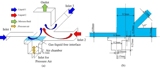
らは大きさσ2の表面張力を持つ液体を流入させることを想定している.このと き,その表面張力の大小関係はσ1>σ2であるとする.合流部には気液自由界面 が設置されるとする. Fig. 2-6に,実際に用いた実験流路の概形を,Fig. 2-7に,実験結果の画像を 示す.実験装置や試験流体は,論文第3章,第4章にて詳述したものを使用した. 実験の結果,この形式の流路において,最大 20.0[s]程度,マイクロ混合流の 生成に成功したが,継続的な混合促進には至らなかった.また,このときの実 験条件では,2 種の実験流体の流入量が等量にならないことも問題となった. Inl e t 3 : Flow of “liquid 1” : Flow of “liquid 2”
: Flow of mixed fluid : Marangoni force [surface tension; σ1(> σ2)] [surface tension; σ2(< σ1)]
: Contact point
between liquid 1 and 2
Inl e t 1 Inl e t 1 Inl e t 2 Inl e t 2 Inl e t 3 Outlet Outlet (a) (b)
: Gas-liquid free interface : Roll flow
27
Fig. 2-6 Details of the junction point in “Type-A” test channel using the flow experiments, (a); Isometric projection drawing with flow pattern of each channel. (b); Front view of orthographic projection drawing with dimensions.
Fig. 2-7 A series of photos of the flow experiment using a test channel described in Fig. 2-6 every 0.1(s) from (a) to (l), volume flow rate; Inlet 1:2.0μl/min, Inlet 2:1.0μl/min and Inlet 3:2.0μl/min [9] 0.3mm 0.1 5 mm 0.3mm 0.2mm 0.04mm 0.15mm 0.08m m 0.05 m m 0. 25 m m 45° 0. 25 m m (b) Inlet 1 Inlet 2 Inlet 3 Outlet Inlet for Pressure Air Air chamber
Gas-liquid free interface
30
(a)
(b)
32
Fig. 2-4 Details of two-dimensional model using the CFD analysis, (a); Overall geometry of the CFD models, (b); Details of the CFD model.
35
第 2 章の参考文献
[1] Incropera, F.P., Dewitt, D.P., Bergman, T.L. and Lavin, A.S., Fudamentals of Heat and Mass Transfer, WILEY, NJ, USA, 2007,
[2] 宗像健三,守田幸路,輸送現象の基礎, コロナ社,2006,pp. 12-51.
[3] 小川浩平,黒田千秋,吉川史郎,化学工学のための数学,数理研究社,2007, pp. 69-108
[4] 吉田純一監修, ”マイクロリアクターの開発と応用”シーエムシー出版,2008. [5] Scriven, L.E. and Sternling, C.V., The Marangoni Effect, Nature, 187, 1960,
186-188.
[6] 今井 功,流体力学(前編),裳華房,1973,pp. 259-399.
[7] Brennen, C.E., Fundamentals of Multiphase Flow, Cambridge University Press, 2005, pp. 30- 67.
[8] 山田 崇,小野直樹,マランゴニ力を活用したマイクロ混合流の生成,日本 機械学会論文集B編 79, 2013,pp888-899.
[9] 山田崇,加藤直毅, 竹田和幹, 小野直樹,「マランゴニ対流を用いたマイクロ
混合プロセスに関する基礎研究」,日本混相流学会年会講演会 2011
[10] Yamada. T and Ono. N, A Study on Micromixing Utilizing Marangoni Effect Induced on Gas-Liquid Free Interfaces, ASME; J. Micro Nano-Manuf. 3(2), 2015, 021003, doi:10.1115/1.4029684
[11] http://www.phoenics.co.jp/
[12] S. V. Patankar, 水谷幸夫, 香月正司 共訳, コンピュータによる熱移動と流 れの数値解析, 1985, 森北出版.
[13] R. B. Bird, W. E. Stewart, and E. N. Lightfoot, Transport Phenomena second edition, 2006,WILEY.
[14] 吉田純一監修, マイクロリアクターの開発と応用,シーエムシー出版,2008. [15] Incropera, F.P., Dewitt, D.P., Bergram, T. L., and Lavine, A. S., 2007, “Fundamentals of Heat and Mass Transfer,” John Wiley and Sons, NJ, USA, pp. 880–897.
40
41
43
でΔV / V を-7.1×10⁻⁴に,約 1/2 回転(約 180°)でΔV / V を-7.1×10⁻³に到
達させることが可能になる.上記の理論的背景から,この手動制御(Manual Drive)シリンジドライバを用いることにより,実験時において,気相内内圧 を適切に制御することが可能になった.
Fig. 3-2 Diagram of the air pressure control system
Fig. 3-3 Schematic view of air pressure control device, (a) general construction, (b) control mechanism of the air pressure
Air Supply and Control
System
Test section
(Micro channel)
Silicon Tube (φ 0.5mm) Gas‐tight Syringe (capacity : 1.0ml) Piston + Spring M12 Fine threadPressure plate Pressure plate Pressure plate
44
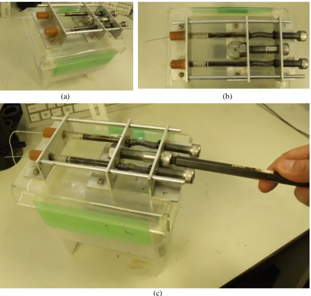
Fig. 3-5 Photos of manual drive air pressure control device, (a)(b) general construction, (c) the operation procedure
(a) (b)
46
PDMS は,多くの工業(潤滑剤,(紙,繊維の)防水加工,防泡剤など)で
大量に使われており,その一般化学式は以下の通りである.
(CH3)3Si‐O‐[(CH3)2SiO]n‐Si(CH3)3
48
Fig.3-6 Schematic view of photolithography process, exposure→developing →casting by PDMS →construction of the test channel
Fig. 3-7 Photos of the mask alignment device, (a) a general view, (b) with a photo mask pattern
Photo mask Silicon wafer
Photopolymer
Silicon wafer
Silicon wafer Grass plate
Micro structure
Micro channel
49
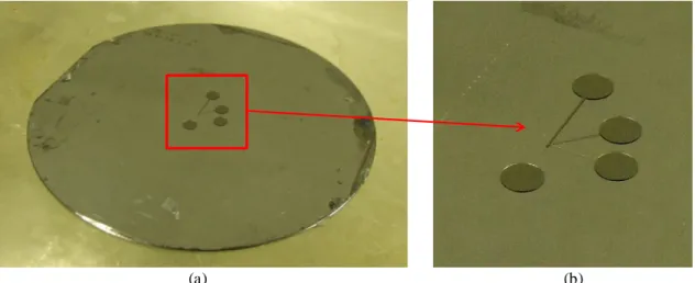
Fig. 3-8 the micro structure of the mold of the test channel on a silicon wafer made by photolithography method, (a) a general view, (b) a enlarged view
Fig. 3-9 Photos of the casting of the micro structure made by photolithography method, (a) a general view, (b) work on detachment process
(a) (b)
50
実際に実験で用いた流路の形状は,Fig. 3-10 に示す通りである.Fig. 3-10(a) に試験流路の全体形,(b)に流路屈曲部の形状および寸法を示す. マスクパターンは実験流路の CAD データをフィルム上に転写し,現像したも のを用いた.Fig. 3-10(c),(d)に,フォトリソグラフィーを用いて作成した試験 流路をレーザー顕微鏡(Olympus LEXT4000)にて測定した結果を示す.流路の 深さ方向が大体 100μm,平面方向の各寸法がマスクパターン通り転写されてい ることが分かる. (a) (b) (c) (d)
Fig. 3-10 The design of Type-B channel, (a) Schematic view of the general construction, (b) Detail of the bending point of Type-B channel including bubble holding section as air-chamber and air-channel, (c)The measuring result of PDMS rubber installing Type-B channel by ×10 of laser micro scope
52
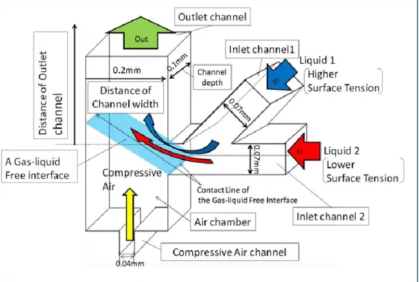
Fig.3-11 Concept of “Micromixer with Thin Liquid Film” (a) The detail of “Bubble holding section” (b) The image of the mixer (c) Important effects in mixing near the bubbles : (1) Decreasing diffusive distance between two bubbles and (2) ambient flow change near the bubble [5]
Fig.3-12 Parameters put into the bubble holding section [5]
53
Fig.3-13 Schematic view of dimensions in the three test channels (a) Over all dimension of test channel, (b) Different designs of “bubble holding section”: (1) Type-A, (2) Type-B and (3) Type-C[5]
三種類の流路は Fig. 3-13(a)に示すとおり,基本的に流路幅 0.15mm,奥行き 0.1mm,主流路に対する Inlet の角が,水平線に対してそれぞれ 45°の Y 型ミ キサーであり,2 液合流部から 3mm 地点に,Fig. 5(b)に示す気泡保持部を設け る.気泡保持部の 3 つのパラメーターについては表 3-1 にある通りである.
Table 3-1 Dimensions of the bubble holding section in different test channels[5]
Test channel Chamber width Chamber depth Distance
54
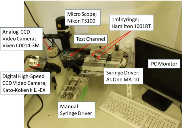
され,流路内に圧縮空気を供給,気泡形状の制御を行う.観察部,記録部は倍 率 4~10 倍の光学顕微鏡,アナログ CCD カメラ,モニター,PC からなり,実 験映像の観察,動画での記録を行った.実験に用いる流体は 25℃の純水を用 いる.流入条件については表 2 に示す.
Fig.3-14 Schematic view of the experimental apparatus[5]
Table.3-2 Flow condition after the junction point in the experiments[5] Volume flow rate
(μl/min) Flow velocity (m/s) Reynolds number
1.0 1.11×10⁻³ 0.17
Type-A,B,C 試 験 流 路 を 用 い た 気 泡 形 成 実 験 の 結 果 を そ れ ぞ れ Fig. 3-15(a),(b),(c)に掲載する.
56
58
第 3 章の参考文献
[1] de Gennes, P.G., Brochard-Wyart and F.B., Quere, D., 奥村剛訳,表面張力の物 理学,吉岡書店,2003,pp. 1-83.
[2] 吉田純一監修, ”マイクロリアクターの開発と応用”シーエムシー出版,2008. [3] Kazawa, E., Ueno, T. and Shinoda, T., High-aspect-ratio lithography for micro module fabrication, Bulletin of Tokyo metropolitan industrial technology research institute, 5, 2002.
[4] http://microchem.com/pdf/SU-8%203000%20Data%20Sheet.pdf.
[5] Yamada, T. and Ono, N., A Basic Study of a Straight Flow Micromixing Device Utilizing a Very Thin Liquid Film, Journal of Fluid Science and Technology 7(1), 2012, pp. 64-77.
61
実験の状況を観察し画像または映像で記録するセクションは,光学顕微鏡, アナログカラ―CCD カメラ,デジタル(モノラル)高速度カメラ,外部 LED 光源,PC,モニターにて構成されている.
光学顕微鏡 (Nikon TS100) には,4 倍 (Nikon CFI Plan Fluor 4x, NA; 0.13), 10 倍 (Nikon CFI Ph1 DL 10x, NA; 0.25),20 倍が二種類 (Nikon CFI Plan 20x, NA; 0.45),(Nikon CFI Plan Apo λ 20x,NA; 0.75) 各レンズが装着されており,目 的に応じて(混合濃度測定,或いは流れの可視化実験)使い分けている(Fig, 4-4 参照). アナログカラ―CCD カメラ (Vixen C0014-3M) は 41 万画素の 1/3 インチカ ラーCCD センサーを備えており,1 秒間あたり 30 コマ (30[fps]) 撮影できる. アナログカラ―CCD カメラは,実験状況の確認,実験結果の撮影に用いてお り,光学顕微鏡 (Nikon TS100)のカメラ塔に装着され使用される.
62
Fig. 4-1 Diagram of the apparatus for the experiments; Overall structure of the apparatus
Fig. 4-2 a photo of the apparatus for the experiments; general construction
Liquid Supply
1ml syringe×2+ Syringe driver
Air Supply and Control
1ml syringe×1 +
63
Fig.4-3 Details of installation of a test channel in the apparatus
Fig. 4-4 Microscope objective lens, (a) 4×(Nikon CFI Plan Fluor 4x, NA; 0.13), (b) 10×(Nikon CFI
Ph1 DL 10x, NA; 0.25), (c) 20×(Nikon CFI Plan 20x,NA; 0.45),(d) 20×(Nikon CFI Plan Apo λ 20x,
NA; 0.75), (e) The microscope (Nikon TS100) mounting these lenses (a) (b)
Rubber tube to the inlet of test channel
Inner diameter; 0.7mm
Grass base Thickness; 0.17mm
The PDMS base of the test channel
Thickness; 3.0mm Rubber tube to the air inlet
Inner diameter; 0.5mm
(a) (b) (c) (d)
64
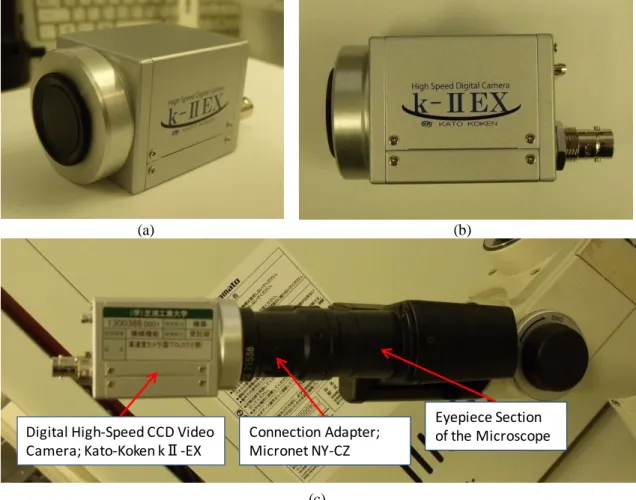
Fig. 4-5 Details of digital CCD high-speed camera (Kato ko-ken kⅡ-EX), (a)(b) general view, (c) connection to the eyepiece barrel of the microscope
Eyepiece Section of the Microscope Connection Adapter;
Micronet NY-CZ Digital High-Speed CCD Video
Camera; Kato-Koken kⅡ-EX
(a) (b)
67
Table 4-2 Values of surface tension, viscosity and contact angle in acetic acid solution[1,12]
Test fluids Density
(kg/m3)
Surface tension (N/m)
Viscosity (Pa・s)
×10-3 ×10-3 ×10-3
Pure water blue dye 1.4wt% dissolved
0.997 69.0 0.96
Acetic acid 30wt% solution 1.035 44.6 1.54
Concentration (wt %) Surface tension (N/m) Contact angle (degree) Viscosity (Pa・s)
68
4-3 混合評価法
4-3-1 酢酸水溶液の拡散に対する混合評価法の検討
本研究では基本的に純水と酢酸 30wt%水溶液の 2 液間の混合を扱っている. 一方,その混合評価に対するトレーサーとして,どちらかの試液に青色食用色 素(Brilliant Blue FCF 8% + Dextrin 92%)を 1.4wt% 添加したものを用いてい る. 純水と酢酸 30wt%水溶液間の拡散係数 D は,20℃において, D=1.24×10⁻⁹ [m2/s] である. 一方,青色食用色素本体(Brilliant Blue FCF)の拡散現象は,純水を溶媒と した色素の拡散であると考えることができる.青色色素である Brilliant Blue FCF の実効濃度は 1.4%×0.08=0.112%であるので,十分希薄濃度と考えること が出来る.希薄溶液中の拡散係数 D はストークス・アインシュタインの式か ら導かれた以下の Wilke and Chang の実験式である式(4-1)から求められる[14].
…(4-1) このとき, ψB:会合パラメーター(水の場合 2.6),MB:溶媒分子の分子量[g/mol] T:温度[K],μ:粘性係数[Pa・s] A V~ :大気圧下の沸点における成分 A の分子容量[cm3 /mol] である.
20℃のとき純水(H2O)中における Brilliant Blue FCF(C37H34N2Na2O9S3)の
69 また,色素の拡散を用いて混合度合いを判定する手法は,Hessel らの論文に て,「最も簡便に混合効果を判定する手法」として紹介されており,一般に用 いられている手法の一つであると認識される[13]. 4-3-2 評価手法概要 マランゴニ対流によるマイクロ混合流による混合評価には,純水に食用色素 を添加した水溶液を用いた流動実験において,その実験画像の輝度を測定する ことにより行った.純水に青色食用色素をトレーサーとして 1.4wt%混入させ た液体は,Table 4-1 にある通り,その密度,粘性係数,表面張力が純水のそれ と大差がないことがわかる. 実験画像の輝度測定手法として,画像解析ソフト”Image J”[2]を用いた画 像内輝度値計算を行った[3]. 実際の手順は,Fig. 4-6 にあるとおり,まず”Image J”を用いて,実験画 像の RGB 分割を行う.赤,緑,青各成分の輝度値に基づいて二値化された三 枚の画像が得られる.そのうち,赤色の輝度について二値化した画像を用いて 輝度値の計算を行った. 測定範囲の輝度値の「最大値」と「最小値」の差分を「最大輝度差」とし, 二液が接触していない部分での 2 液間の輝度差を基準として正規化を行い,混 合進展の指標とした. 「 最 大 輝 度 差 」 は 本 論 文 に 掲 載 し て い る グ ラ フ 中 で は "Relative Concentration Difference",或いは,"Maximum concentration difference"と表記して
70
Fig. 4-6 The process of the luminance measurement evaluating the efficiency of the micromixing flow used by a image processing software “Image J”
Using image analysis program ”Image J”
RGB divided Red Green Blue Brightness(gray scale) in a domain surrounded with a yellow line
71
4-4 PIV(粒子画像化速度計測法)の概要と本研究における適用
Particle Image Velocimetry(PIV.日本語では粒子画像流速計測法と呼ばれる.)
72
Fig. 4-7 Classification scheme for PIV analysis[6]
PIV
Particle Streak Velocimetry
Particle Tracking Velocimetry
Image correlation Method
Laser Speckle Velocimetry Holographic PIV
4-time Tracking Velocimetry Binary-image Correlation Method
73
4-4-1 粒子追跡法
74
一方,一つの理想的な粒子像をテンプレートとしてあらかじめ準備し,粒子 画像の中からテンプレートに類似した領域を粒子像として抽出する方法もあ る.その手法の中から,ガウス分布のテンプレートを用いる粒子マスク相関法 (particle mask correlation method)[7] について述べる.
76 4-4-2 画像相関法 画像相関法は,可視化画像の局所的輝度値パターンの移動量を求めることに より速度ベクトルを測定する手法であり,異なる二時刻間の画像で輝度値パタ ーンの類似度の高い部分を対応付けるものである.この解析手法の持つ最大の 特徴は,流れの可視化法や解析パラメーターの設定などの自由度が比較的高く, 可視化対象に対する応用範囲が広い点である.例えば,この手法では個々のト レーサー粒子像ではなく輝度値パターンの移動を求めるため測定点が任意に 設定でき,渦度・せん断応力等を求める測定結果の後処理に便利なように正方 格子状の測定点を設定することが画像解析・計測の段階で可能である.画像相 関法では 2 枚の瞬間照明された可視化画像が用いられるが,これらの画像が取 り込まれる時間間隔の間に輝度値パターンが大きく変化しないことが解析の 前提になる.ここでは,画像相関法の一方法である,①「直接相互相関法」と ②「再帰的相関法」について,その概要を述べる. ① 直接相互相関法 ・測定原理
77 実際に取り扱う原関数 f, g は連続的には与えられないので,次の離散表現の 定義式で相互相関関数を計算する.但し,検査領域サイズを N×N [pixel] とす る.
N i N j j i j i fg X Y f X Y g X X Y Y C 1 1 , , , …(4-4) また,相互相関をとるとき,値域が[-1, 1]の範囲をとる次の相互相関係数で 評価することも多い
N i N j N i N j m j i m i i N i N j m j i m i i fg g Y Y X X g f Y X f g Y Y X X g f Y X f Y X R 1 1 1 1 2 2 1 1 , , , , , …(4-5) ただし,fm, gm は,それぞれ第 1, 2 画像における N×N の検査領域内の輝度 値パターン f, g の平均値を表す.また,上式にて,fm = gm = 0 とする相互相関 係数の定義式を用いることもある. Fig. 4-8 に直接相互相関法による輝度値パターン移動量検出の概略を示す. 最初に第一画像における任意の位置 A を中心とする N×N の検査領域 (inspection domain)を設定する.次に,第二画像の中に同じ位置 A を中心とする Ns×Nsの領域を探査領域(Detection target domain)として設ける.探査領
78
Fig.4-8 estimation process of "direct cross-correlation method"[5]
80 この相関ピーク位置を求めるために,ピーク値を中心とする三つの相関値にガ ウス分布や二次曲線を当てはめてその極大値位置を求めるか,重心を計算する. 相関ピーク値で得られる整数画素単位の移動量を i とすると,ガウス分布,二 次曲線,重心によるサブピクセル移動量 Psubは,相関値 R を用いてを用いて それぞれ次のように与えられる. ガウス分布 1 1 1 1 ln ln 2 ln ln ln 2 1 i i i i i sub R R R R R i P …(4-7) 二次曲線 1 1 1 1 2 2 1 i i i i i s u b R R R R R i P …(4-8) 重心
1 1 1 1 1 1 i i i i i i s u b R R R R i iR R i P …(4-9) 上記の式に従い,X 方向移動量,Y 方向移動量それぞれ別々にサブピクセル 移動量 Psubを求め,これにより 0.1pixel の精度で輝度値パターンの移動量を測 定することが出来る.Fig. 4-9 estimation process of "sub-pixel precision" for Gaussian distribution [6]
X
i-1 i i+1
Psub
; The peak value in the pixel unit position
82 (2) 誤ベクトルの除去を行う.このとき,誤ベクトルが残らないように注意 する必要がある.さらに,除去された誤ベクトル位置におけるベクトルを補間 して求め,ベクトル候補とする. (3) 検査領域サイズを一回り小さくする(例えば 32×32[pixel] など)ととも に,探査領域をステップ(2)で求められたベクトル候補の周囲に限定する.探 査領域を限定することで,小さな検査領域でも誤ベクトルの発生を抑えること が出来る. (4) ステップ(2)と(3)を繰り返す.このことで,検査領域サイズはどんどん小 さくなるが,誤ベクトルの発生も抑えられる. 検査領域の縮小を再帰的に行うことから,再帰的相関法,階層的相関法 (hierarchical cross-correlation method)などと呼ばれる .
83 後の主流となると考えられる.なお,粒子密度以上のベクトルが求められたと しても,それはベクトルを空間補間していることに注意する. ③ 回転,変形を考慮した画像相関法 画像相関を用いる手法は,輝度値パターンの画像相関や差の絶対値を用いて 比較を行っている.このとき,検査領域と,その相手側(候補領域)として小 領域を取り出している.画像相関法では,輝度値パターンの比較は単純に並行 移動を仮定して求められている.しかしながら,微小時間の間にも流体は変形 したり回転したりしている.このような流体の変形や回転を考慮する為には, 従来は粒子追跡法(PTV)に頼らざるを得なかった.粒子追跡法では,並行移 動のみではなく回転や変形にも考慮しているが,輝度値パターンの並行移動を 本質的に仮定している画像相関法では,大きな変形がある場合には誤差が大き くなってしまう.そこで,回転(rotation)や変形(trans-formation)が考慮さ れる画像相関法が開発された[10].
Fig. 4-10 correlation method considering for rotation or transformation of the fluid
再帰的相関法を用いることで,空間的に解像度の高いベクトルを得ることが 出来る.この得られたベクトルは,検査領域の並行移動を仮定して求められて いる.ある検査領域に着目すると,この検査領域の周囲で得られているベクト ルを参照することで,検査領域の回転や変形行列を算出することが出来る.1 時刻目の検査領域をこの回転変形行列によって変形させたものを計算する.そ の概略を,Fig. 4-10 に模式的にしめす.Fig. 4-10 の点線領域に示す,この変形 後の検査領域と 2 時刻目の対応領域とを用いて,画像解析を行い詳細な移動先 を決定する.なお,この移動先はサブピクセルの決定に用いられる. なお,変形後の画像と 2 時刻目の画像の相関を計算する場合には,画素ごと の計算を実施する必要がある.一般に変形後の画素位置は,ずれているため, 画像補間によって各画素位置における変形後の輝度値を算出する必要がある. 画像を変形させているため,より精度の高い解析が行えるとされている.この Rotation
Transformation Image Correlation
85
の輝度差から,PIV 解析にも耐えうる画像が得られると考えられる.
また,高輝度の可視連続光の照射方向は,顕微鏡レンズの入射方向に正対し ているので,PIV 観察断面の厚さ(thickness)は,通常の顕微鏡観察による 被 写界深度(焦点深度)(Depth of Field; DOF)から決定されると考えられる.
被写界深度(焦点深度)を計算する理論式はいくつか提案されているが,そ の中に,(4-10)式に示す Martin の式 (Martin's equation) がある.
mNA NA n DOF 2 7 1 …(4-10) 但し, λ;可視光の波長 NA;顕微鏡レンズの開口数 m;顕微鏡レンズの倍率 n;媒質の屈折率 式 (4-10) は,「物理学的焦点深度」と「幾何光学的焦点深度」の和として表 現されている.「幾何光学的焦点深度.は,肉眼での観察のときに,人体の眼 の焦点の限界により問題となる要素であり,CCD カメラによる PIV 解析画像 の撮影に関しては,「物理学的焦点深度」のみがパラメーターとして重要にな ると考えられる.この点を考慮して式 (4-10)を書き直すと,式 (4-11) のよう になる. 2 NA n DOF …(4-11) 式 (4-11) から,比較的 NA 値(開口数)の大きなレンズを本研究に用いる (第 4 章 4-1Fig. 4-4(b)~(d)参照)ことにより,その被写界深度(焦点深度)を 数 μm~十数 μm 程度にすることが可能となり,極めて薄い流体断面の解析画 像を得ることが出来ると考えられる. 以上の理由により,本研究ではその可視化光源として高輝度の可視光を用い ている.
可視化光源は,Fig. 4-12(a)に示す通り,高輝度 LED 可視化光源 LA-HDF158AS
86
色温度は 600,000[Lux]に達する.この可視化光源を用いることにより,ハイス ピードカメラのシャッタースピードを 1/21,000[1/s]の条件で撮影することが可 能となった.この光源を,長さ 1.0m のエクステンションにより,試験流路直 上まで導いて実験流路上に照射している(Fig. 4-12(b),(c)参照).
Fig. 4-11 relationship between the optical system of visible light and depth of field in the experiment apparatus
87
(a) (b)
(c)
Fig. 4-12 photos of the experiment apparatus for PIV measurement, (a) LED lighting system LA-HDF158AS (Tokyo Grass, Co.LTD) (b) general construction using LED lighting system, (c) detail of the experiment system using extension end of the LED lightning system
本研究では,取得画像から PIV 解析によりベクトル量を算出し,その流れ 速度を解析する為に,Flow Expert 2D2C(カトウ光研)という PIV 解析ソフト ウェアを用いた[11].
Digital High-Speed CCD Video Camera; Kato-Koken kⅡ-EX
88 Flow Expert 2D2C は,上述した直接相互相関法,再帰的相関法,画像変形法 による PIV 解析が可能であり,粒子追跡法(PTV)による解析(2 値化相関法, 粒子マスク相関法)にも対応する.また,誤ベクトルの除去,補間やサブピク セル解析に対しても対応している.以上から,本研究で扱う流体内の変形量が 大きいことが予想される流れ分布の解析に対応し得ると考えられるため,これ を採用した.本研究における PIV 解析では,これら,直接相互相関法,再帰 的相関法,画像変形法そして粒子追跡法を,適宜使い分けている. 本研究で用いる PIV システムの測定精度についてであるが,本研究で用い た PIV ソフトウェアは,直接相互相関法については,相互相関関数に加えて サブピクセル補間まで行っているため,0.1 ピクセルまでの分解能を持ってい ることになる.これは,1 フレーム当たりのトレーサー1 個当たりの移動距離 の適正値といわれる 5~7[pixel]に対して約 2%の分解能を持っていることにな る.したがって,この条件下では,測定精度 2%以下ということになる. 本実験系に対しての測定精度を確認するため,実験流路内における純水とト レーサー粒子(0.1wt%添加)の組み合わせによる流動観察を行った.これは 流路幅 0.2mm,流路深さ(流路平面形に対する)0.1mm の直線流路を用いて 行った.実験流路は第 3 章 3-3 で述べた方法にて作製,構成された流路を用い た.流入条件は,体積流量 3.0[μl/min]( 5.0×10-11 [m3/s]),顕微鏡レンズ倍率 20 × (NA: 0.75),撮影条件は 1000[fps]とし,このときの 1[pixel]当たりの相当距離 は約 0.5[μm]であった.PIV 解析は,再帰的相関法(hierarchical cross-correlation method) を用い,サブピクセル解析以外の補間方法は一切行わなかった.
89
Fig. 4-13 the dimentions of the CFD model compared with the result of PIV analysis, volume flow rate flom inlet;5.0×10⁻¹¹[m3/s]
Fig. 4-14 (a) contour views of the CFD result, above; Z-X plane , bellow; X-Y plane
90
Fig. 4-15 the result of PIV analysis compared with CFD result of X-Y plane (Z=0.05mm)
92
第 4 章の参考文献
[1] 山田 崇,小野直樹,マランゴニ力を活用したマイクロ混合流の生成,日本 機械学会論文集B編 79, 2013,pp888-899.
[2] http://imagej.nih.gov/ij/
[3] Yamada, T., Watanabe, Y., Osato, N., and Ono, N., Experimental and Numerical Study on Micromixing utilizing Movement of Gas - Liquid Free Interface, Journal of Fluid Science and Technology, 6(2), 2011, pp.128-138.
[4] de Gennes, P.G., Brochard-Wyart, B.and Quere, D., 奥村剛訳,表面張力の物理 学, 吉岡書店,2003,pp. 1-83.
[5] Ehrfeld, W., Golbig, K., Hessel, V., Löwe, H. and Richter, T., Characterization of Mixing in Micromixers by a Test Reaction:Single Mixing Units and Mixer Arrays, Ind. Eng. Chem. Res. 38, 1999, pp.1075-1082.
[6] (社)可視化情報学会編,PIV と画像解析技術,朝倉書店,2004,pp. 1-46. [7] (社)可視化情報学会編, PIV ハンドブック,森北出版,2002,pp.69-103. [8] 竹原幸生,江藤剛治,道奥康治,久野悟志,粒子マスク相関法の性能評価,
可視化情報,vol.17, Suppl. No1, 1997, pp. 117-120.
[9] M. Raffel, C.E. Willert and J. Kompenlans, Particle image velocimetry, a particle guide, Springer-Verlag, 1998.
[10] 北洞貴也,笠原鋼一,黒川淳一,松井純,画像変形方式 PIV 法の提案,可視 化情報,vol.19, Suppl, No 1, 1997.
[11] http://www.kk-co.jp/detail/flowexpert_.php
[12] Washburn, E. W., International Critical Tables of Numerical Data, Physics, Chemistry and Tecnology, vol.5.
[13] Hessel, V., Löwe, H. and Sohnfeld, F., Micromixers – a review on passive and active mixing principles, Chemical Engineering Science 60, 2005, 2464-2501.
94 5-1 実験概要 5-1-1 実験条件の設定 混合流生成実験の実験条件について説明する. 実験流路の外形と,2 試液合流部の平面図を Fig. 5-1 に示す.混合流生成実 験では,第 2 章 2-3 で述べた通り,第 3 章 3-3 で示した実験流路内に,第 4 章 4-1,4-2 でそれぞれ説明した実験装置と 2 試液を用い,表面張力値の異なる 2 液を気液自由界面上で合流させることでマランゴニ対流によるマイクロ混合 流を生成させる.しかし,Fig. 5-1 に示す二つのインレット,即ち Inlet 1, Inlet 2 に対して,実験で用いる 2 試液のうち,どちらにどの試液を用いるか(流入 させるか)で,実験開始時のマランゴニ対流発生の方向が異なり,それが実験 流路内主流に及ぼす影響についても相違すると考えられる.
Fig. 5-2(b)に,Inlet 1 に純水,Inlet 2 に酢酸 30wt%水溶液を流入させたとき に予想される,気液自由界面上の表面張力分布の概形と,マランゴニ対流の発 生方向について表す.マランゴニ対流は,表面張力値が小さいほうから大きい ほうへ向けて発生するものなので,マランゴニ対流は「流路内主流に対して順 方向に.発生する.これは,Fig. 5-2 (a)に示すとおり,気泡周辺の流れは,気 泡表面の一点に引力が生じるように影響を受けていることが分かる.これによ り,管内主流の流線が歪むので,これによる混合効果の増加が期待できる.し かし,気液自由界面上に発生するマランゴニ対流が,管内主流に対して十分に 大きくなければ,マランゴニ対流は実質上,管内主流の平面内速度分布内に埋 もれる形となり,十分な混合促進効果を持たなくなる恐れがある.
95 本論文中では,Fig. 5-2 に示す,実験初期にマランゴニ対流が「流路内主流 に対して順方向に」発生すると思われる条件については,実験条件「Case 1」, Fig. 5-3 に示す,実験初期にマランゴニ対流が「流路内主流に対して逆方向に」 発生すると思われる条件については,実験条件「Case 2」として定義し,以後, 実験結果の整理・区別,考察等に用いることとする. (a) (b)
Fig. 5-1 the test channel, (a) General view, (b) Detail of dimensions in the bending point including bubble holding section as air-chamber and air-channel
96
(a) (b)
Fig. 5-2 (a) Stream line near a spherical bubble in constant flow of horizontal direction with surface tension gradient with the Marangoni force at follow direction to the constant flow (b) The experimental system for the flow experiment with Marangoni convection at follow to the main flow direction in initial condition
(a) (b)
Fig. 5-3 (a) Stream line near a spherical bubble in constant flow of horizontal direction with surface tension gradient with the Marangoni force at against direction to the constant flow (b) The experimental system for the flow experiment with Marangoni convection at against to the main flow direction in initial condition
99 = {(Δσx/μD)( μ/ xρv) ( D/ xv)} π1{μ/( xρv)} π4{ (Dρ/μ)( μ/ρx v)} π6 = {(Δσx/μD)( μ/ xρv) (Dρ/μ)( μ/xρv)} π1{μ/( xρv)} π4{ (Dρ/μ)( μ/xρv)} π6 …(5-6) 以下のように定義される無次元数 Marangoni 数 Ma =Δσx/μD Reynolds 数 Re = xρv/μ Schmidt 数 Sc = μ/ Dρ から,式(5-6)は,次の式(5-7)のように変形される.
= {Ma・Re-2・Sc-1 } π1{Re-1} π4{ Sc-1・Re-1} π6 …(5-7)
100 5-2-2 実験系を支配する無次元数と主要パラメーター 本研究に用いた実験系は,第 5 章 5-2-1 で実施した次元解析において, ・Marangoni 数(Ma=Δσl/μD), ・Reynolds 数(Re=ρul/μ), ・Schmidt 数(Sc=μ/ρD), が支配する系として導かれた. このうち,Marangoni 数はマランゴニ効果を支配する無次元数として知られ ており,ある臨界値を超えると対流は定常流から振動流に移行することが知ら れている[9]. Reynolds 数は流体の流れを支配する無次元数として知られており,臨界値 を超えると流れは層流から乱流に移行することが知られている[10]. Schmidt 数は,流れと物質移動の関係を定める因子であり,流体の物性だ けで決まる物性値である[10]. これらの無次元数は,表面張力差Δσ,液相内主流の速度 u,液相内の粘度 μ,, 純水-酢酸水溶液間の拡散係数 D,流路内代表長さ l,以上をパラメーターとし て用いることにより得られる. 実験中では,流入条件は体積流量により管理されている.実験においては,
実験条件「Case 1」,「Case 2」を通じて,概ね一インレット当たり 0.5μl/min か
ら2.5μl/min までを用いている.このとき,流路平面内の流路幅 l1(第 2 章 Fig.
内の"channel width")を代表長さに取った Reynolds 数(Re)を考えると,体積 流量は一定であり,また,平面内の流路幅は場所によって異なるが,流路奥行 き方向の長さ l2(第 2 章 Fig. 2-8(a) 内の"channel depth")は,常に一定である.
101
5-3 流れと同方向に生じるマランゴニ力による混合流生成実験
5-3-1 流入条件と主要パラメーター
実験時に採用した流入条件を Table 5-1 に示す.
Table 5-1.Flow condition at each inlet in the experiments[1,4] Volume Flow Rate
(μl/min)
Reynolds Number (Pure water)
Reynolds Number (Acetic acid solution)
0.5 0.08 0.06 0.8 0.13 0.09 1.0 0.17 0.11 本実験系は,第 5 章 5-2-1 から,本実験系においては, ・Marangoni 数(Ma=Δσl/μD), ・Reynolds 数(Re=ρul/μ), ・Schmidt 数(Sc=μ/ρD), が支配する系として導かれた. これらの無次元数は,表面張力差Δσ: 0.1~23.0 [N/m](23.0 [N/m];酢酸 15[wt%] 水溶液と純水の表面張力値の差),液相内主流の速度 u: 2.38~11.90×10⁻³ [m/s], 液相内の粘度μ : 1.38×10⁻³ [Pa・s](酢酸 15[wt%]水溶液の粘度),密度ρ: 1000 [kg/m3](純水と酢酸水溶液では,ほぼ一緒),純水-酢酸水溶液間の拡散係数 D: 1.24×10⁻⁹ [m2/s],流路内代表長さ l: 7.0×10⁻⁵[m](流路合流部入り口流路幅)
を採用して,本実験系での代表する無次元数 (Referenced dimentionless number) を計算すると,その範囲は Table 5-2 に示すようになる.
Table 5-2.The relations between the range of dominant dimensionless numbers and the condition of the main parameters in the experiment system
104
Fig.5-4 vertical cross-sectional views of the flexion area in the L-shaped region of the three test channels, (a) Type-A, (b) Type-B, (c) Type-C [1]
(a)
(b)
(c)
105
5-3-3 混合評価実験
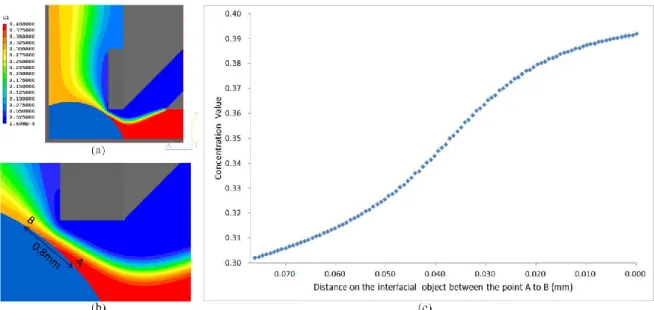
Fig. 5-5,6,7 に,Type-A,B,C 各実験流路において,両インレットの体積流量を 各 0.8[μl/min] (Ma=940860.2, Re=0.192, Sc=1112.9) として行った混合評価実験 の結果をそれぞれ示す.各流路の L 型屈曲部内での,酢酸水溶液と着色純水 の挙動を 0.1 秒毎に比較した. Fig. 5-8,9,10 は,Type-A,B,C 各実験流路において,流路屈曲部を起点に,そ の部分から下流部における流路各地点における二液の混合状態をそれぞれ記 録した画像である. Fig. 5-11 は Fig. 5-8,9,10 で表した画像から,アウトレット流路各地点におけ る 2 液間の青色色素の最大濃度差をプロットしたものである.2 液間の最大濃 度差は,第 4 章 4-3 で述べた通り,実験画像の輝度の RGB 値の R(レッド) 値を比較することで得ている.
Fig. 5-12 は,Fig. 5-8 のうち,Fig. 5-12(a)で示す,流路屈曲部から 0.5mm 地 点でのアウトレット流路上の流路断面方向 A-B の二液間の濃度分布をプロッ トしたものである[1-3,5-6]. 実験の結果,Fig. 5-5 から,気泡による混合デバイスを持つ実験流路では, 気液自由界面形成後,ゆっくりと気泡内圧を上げていったところ,界面の頂点 と流路屈曲部角との距離が 30μm 以下となったと思われる時点で界面と界面 周辺で流れが周期的に強く駆動され,これにより混合が大きく促進している様 子が見られた.そしてこの状態は,曲率半径等,気泡形状が維持されている間, 途切れることなく持続されていた.但し両流路による実験中,シリンジから供 給される試験流体の流れには,脈動のような周期的な流れの変化が表れていた. このような流れの変化は,Fig. 5-6,7 に示す,Type-B,C 流路を用いた流動実験 にはほとんど表れなかった. 今回用いた 2 種の試験流体間の界面張力差により,二液の接触界面の挙動自 体が不安定になったことも脈動流の挙動を助長したと考えられる.また,特に L 字型流路の屈曲部にてその挙動が不安定になったことから,試験流路の物理 的形状もこのような流れの挙動に関係していることも推察される.これは, Type-B,C 流路を用いた流動実験にはほとんど表れなかった.
106
酢酸濃度が厳密に反映させたものでないことを断わっておく.
107
Fig. 5-5 A series of photos at the bending point of the test channel in a flow experiment every 0.1 s from (a) to (j) using "Case 1" condition on Type-A channel, volume flow rate; 0.8 μl/min in each inlets, (Ma=940860.22, Re=0.19, Sc=1112.90) [1,5].
Fig. 5-6 A series of photos at the bending point of the test channel in a flow experiment every 0.1 s from (a) to (j) using "Case 1" condition on Type-B channel, volume flow rate; 0.8 μl/min in each inlets, (Re=0.19, Sc=1112.90) [1,5].
Fig. 5-7 A series of photos at the bending point of the test channel in a flow experiment every 0.1 s from (a) to (j) using "Case 1" condition on Type-C channel, volume flow rate; 0.8 μl/min in each inlets, (Re=0.19, Sc=1112.90) [1,5].
0.15mm
0.15mm
108
Fig. 5-8 A series of photos at each point of outlet channel between 0.0mm and 3.0mm from the bending point in the test channel in a flow experiment using "Case 1" condition on Type-A channel, volume flow rate; 0.8 μl/min in each inlets, (Ma=940860.22, Re=0.19, Sc=1112.90) [1,5].
Fig. 5-9 A series of photos at each point of outlet channel between 0.0mm and 3.0mm from the bending point in the test channel in a flow experiment using "Case 1" condition on Type-B channel, volume flow rate; 0.8 μl/min in each inlets, (Re=0.19, Sc=1112.90) [1,5].
Fig. 5-10 A series of photos at each point of outlet channel between 0.0mm and 3.0mm from the bending point in the test channel in a flow experiment using "Case 1" condition on Type-C channel, volume flow rate; 0.8 μl/min in each inlets, (Re=0.19, Sc=1112.90) [1,5].
0.15mm 0.15mm
109
Fig.5-11 Results of maximum concentration difference of blue dye at some distances of outlet channel from the bending point in the test channel in the mixing experiments in Type-A, B and C channels using "Case 1" condition [1,5,7]
Fig. 5-12 (a) Definition of section A to B at the point of 0.5mm of outlet channel from the bending point of the test channel, (b) The result of concentration value of blue dye at some points of section A to B in the mixing experiments using "Case 1" condition(Ma=940860.22, Re=0.19, Sc=1112.90) [1,7] 0.2 0.4 0.6 0.8 1.0 0.00 0.02 0.04 0.06 0.08 0.10 0.12 0.14 0.16 0.18 0.20 C o n ce n tr a ti o n V a lu e o f B lu e D y e
Distance of Channel Width between the point A to B (mm)
(a) (b)
112
Fig. 5-13 The series of high-speed photos, (a) Illustration of the measurement area (inside the frame line), (b) to (i) the PIV analysis of flow velocity at the upstream of the mixing device, volume flow rate; 0.8 μl/min in each inlets(Ma=940860.22, Re=0.19, Sc=1112.90), frames per second; 2000[fps][4]
(a) Measurement Area (b) 0.2655s (c) 0.2675s
(d) 0.2725s (e) 0.2775s (f) 0.2815s
(g) 0.2865s (h) 0.2915s (i) 0.2960s
113
Figure 5-14. The series of high-speed photos, (a) Illustration of the measurement area (inside the frame line), (b) to (i) the PIV analysis of flow velocity at the downstream of the mixing device, volume flow rate; 0.8 μl/min in each inlets(Ma=940860.22, Re=0.19, Sc=1112.90), frames per second; 1000[fps][4]
(f) 0.207s (g) 0.209s (i) 0.219s (d) 0.201s (e) 0.203s (f) 0.205s (a) Measurement Area (b) 0. 194s (c) 0.199s
114
5-4 流れと逆方向に生じるマランゴニ力による混合流生成実験
5-4-1 流入条件
実験時に採用した流入条件を Table. 5-3 に示す.
Table 5-3.Flow condition at each inlet in the experiments
Volume Flow Rate (μl/min)
Reynolds Number (Pure water)
Reynolds Number (Acetic acid solution)
1.0 0.17 0.09 1.5 0.25 0.14 2.0 0.33 0.18 次に,本実験系は,第 5 章 5-2-1 から,少なくとも液相内においては, ・Marangoni 数(Ma=Δσl/μD), ・Reynolds 数(Re=ρul/μ), ・Schmidt 数(Sc=μ/ρD), が支配する系として導かれた. これらの無次元数は,表面張力差Δσ: 0.1~23.0 [N/m](23.0 [N/m];酢酸 15[wt%] 水溶液と純水の表面張力値の差),液相内主流の速度 u: 2.38~11.90×10⁻³ [m/s], 液相内の粘度μ : 1.38×10⁻³ [Pa・s](酢酸 15[wt%]水溶液の粘度),密度ρ: 1000 [kg/m3](純水と酢酸水溶液では,ほぼ一緒),純水-酢酸水溶液間の拡散係数 D: 1.24×10⁻⁹ [m2/s],流路内代表長さ l: 7.0×10⁻⁵[m](流路合流部入り口流路幅)
を採用して,本実験系での代表する無次元数 (Referenced dimentionless number) を計算すると,その範囲は Table 5-4 に示すようになる.
Table 5-4.Relations between the range of dominant dimensionless numbers and the condition of the main parameters in the experiment system
116
5-4-2 混合評価実験
Fig. 5-15 に,両インレットの体積流量を各 1.0[μl/min] (Ma=940860.2, Re=0.24,
117
Fig. 5-15 A series of photos at the bending point of the test channel in a flow experiment every 0.1 s from (a) to (j) using "Case 2" condition, volume flow rate; 1.0 μl/min in each inlets, (Ma=940860.22, Re=0.24, Sc=1112.90)
Fig. 5-16 A series of photos at each point of outlet channel every 0.5mm between 0.0mm and 4.5mm from the bending point of the test channel in a flow experiment of "Case 2" condition, volume flow rate; 1.0μl/min in each inlets(Ma=940860.22, Re=0.24, Sc=1112.90)
118
Fig. 5-17 A series of photos at each point of outlet channel every 0.5mm between 0.0mm and 3.5mm from the bending point of the test channel in a flow experiment of "Case 2" condition, volume flow rate; 1.5μl/min in each inlets(Ma=940860.22, Re=0.36, Sc=1112.90)
Fig. 5-18 A series of photos at each point of outlet channel every 0.5mm between 0.0mm and 4.5mm from the bending point of the test channel in a flow experiment of "Case 2" condition, volume flow rate; 2.0μl/min in each inlets(Ma=940860.22, Re=0.48, Sc=1112.90)
119
Fig.5-19 Results of maximum concentration difference of blue dye at some distances of outlet channel from the bending point in the test channel in the mixing experiments of "Case 2" condition(Ma=940860.22, Re=0.24~0.48, Sc=1112.90)
Fig.5-17 (a) Definition of section A to B at the point of 0.5mm of outlet channel from the bending point of the test channel, (b) The result of concentration value of blue dye at some points of section A to B in the mixing experiments in "Case 2" condition volume flow rate; 1.5 μl/min in each inlets (Ma=940860.22, Re=0.36, Sc=1112.90) 0.40 0.50 0.60 0.70 0.80 0.90 1.00 0.00 0.50 1.00 1.50 2.00 2.50 3.00 3.50 4.00 M ax im u m C o n ce n tr at io n D if fe re n ce o f B lu e D ye Distance (mm) 1.0μl/min 1.5μl/min 2.0μl/min A B (a) (b) 0.00 0.20 0.40 0.60 0.80 1.00 0.0 25.0 50.0 75.0 100.0 125.0 150.0 175.0 200.0 C o n ce n tr at io n V al u e o f B lu e D ye
120
5-4-3 流れ可視化実験
121
ッター速度 1/50000[s])で撮影した.このような実験機材の一部変更を行った 理由として,第 4 章 4-1 で述べたデジタル高速度カメラ kⅡ-EX を用いた場合 には,以下の問題が生じたと思われる.
123
Fig. 5-18 The series of high-speed photos with the PTV analysis of flow velocity every 0.002[s] from (a) to (h), volume flow rate; 2.5μl/min in each inlets (Ma=940860.22, Re=0.60, Sc=1112.90), frames per second; 1000[fps][7]
(a) (b) (c) (d)
124
Fig. 5-19 The series of high-speed photos with the PIV analysis of flow velocity every 0.0033[s] from (b) to (y) at the area in the red frame described in (a), volume flow rate; 2.0μl/min in each inlets (Ma=940860.22, Re=0.48, Sc=1112.90), frames per second; 30000[fps]
125
Fig. 5-20 A high-speed photo (Frame number; 2279) with two velocity vector (Lattice number; 241[bellow] and 272[above]) of a flow visualized experiment with PIV analysis, volume flow rate; 2.0μl/min in each inlets (Ma=940860.22, Re=0.48, Sc=1112.90), frames per second; 30000[fps]
Fig. 5-21 The result of PIV analysis of flow velocity at lattice number 241 (in the red frame area described in Fig. 5-20) of every photo, volume flow rate; 2.0μl/min in each inlets(Ma=940860.22, Re=0.48, Sc=1112.90), frames per second; 30000[fps]
126
Fig. 5-22 The result of PIV analysis of flow velocity at lattice number 272 (in the red frame area described in Fig. 5-20) of every photo, volume flow rate; 2.0μl/min in each inlets(Ma=940860.22, Re=0.48, Sc=1112.90), frames per second; 30000[fps]
![Fig. 1-1 schematic drawing of selected passive and active micromixing principles.[3]](https://thumb-ap.123doks.com/thumbv2/123deta/9766199.1850203/11.892.177.773.588.963/fig-schematic-drawing-selected-passive-active-micromixing-principles.webp)
![Fig. 1-3 a micromixing process utilizing gas-liquid free interface by many bubbles, (a) a image of a flow experiment, (b) experimental and numerical result conpared with conventional micromixer [12]](https://thumb-ap.123doks.com/thumbv2/123deta/9766199.1850203/17.892.155.803.156.410/micromixing-utilizing-interface-experiment-experimental-numerical-conventional-micromixer.webp)
![Table 3-1 Dimensions of the bubble holding section in different test channels[5]](https://thumb-ap.123doks.com/thumbv2/123deta/9766199.1850203/60.892.137.762.148.597/table-dimensions-bubble-holding-section-different-test-channels.webp)