On Misspecified ARMA Model Fittings to Some Stationary Processes

On Misspecified ARMA Model Fittings to Some

Stationary Processes

Minoru Tanaka

School of Network and Information, Senshu University, 2-1-1, Higasimita, Tama-ku, Kawasaki,

Kanagawa 214-8580, Japan

Abstract

This paper gives discussions on (i) a misspecified ARMA(1,1) model fitting to MA(2) processes, and also on (ii) a misspecified MA(2) model fitting to AR(2) processes. They are mainly concerned a problem for finding a number of locally maximal points of the conditional likelihood function of the models when the sample size tends to infinity. It is detected in the case (i) that the general conditions for MA(2) parame-ters on which the conditional likelihood function of the ARMA(1,1) model has more than one locally maximal points in the stationary and invertible parameter space. Also in the case (ii) it is seen that the MA(2) model has three locally maximal points in the invertible parameter space if the model is fitted to special AR(2) processes. These results are inspected by simulation.

Key words: ARMA process; ARMA(1,1) and MA(2) model fitting; conditional likelihood function; locally

minimal points; misspecification.

1. Introduction

This paper is a sequel of the paper [11] last year. It relates to incorrect identification of an ARMA(1,1) model. We treated applying this model to the time series which follows AR(2) process incorrectly. We searched for the conditions of the coefficient parameters of AR(2) process in which two or more maximum points exist in quest of a conditional likelihood function paying attention to the number of the maximum points there. The following graphs of the domain is obtained.

Figure 1. The region of an ARMA(1,1) parameters where more than one locally maximum points exist.

This is also a sequel of the paper "On a moving average time series model fitting" contributed with Mr. Kenji Aoki in 1991 ([12]). It is known that when we fit an MA(1) model to some special time series data which does not follow MA(1) process, the MA(1) parameter does not have an unique Gaussian quasi-maximum likelihood estimator. Tanaka and Huzii [13] have given the conditions of AR(2) parameters on which the MA(1) quasi-likelihood function has more than one local maximal points in the invertible parameter space (-1,1). Furthermore, Tanaka and Aoki [12] gave the region for the AR(2) parameters on which the MA(1) quasi-likelihood function has more than one local maximal points in the parameter space. In this case, maximizing the likelihood function is equivalent to minimizing the following function S(x; a, b) when the data length is large (see [13]). Here x is an MA(1) parameter and a and b are AR(2) parameters.

Sx; a, b =

_{1-b 1-a}1+b-a2_{+2 b+b}1-b x-b 1+b x2_{ 1-x}2_{ 1+a x+b x}2 2_

.

(1.1)

From Tanaka and Huzii [10], we have two minimal points of the function S(x;a,b) = S(x), say. For exam-ple, in the case of an AR(2) process with a = -0.1, b = 0.8, the function S(x) has a graph shown in the following figure. In order to have the conditions on which the function has two local minimal points in the parameter space, we should consider the differentiation DS(x) = 0. And we specified the case where the solution of the equation DS(x) = 0 changed from three to two. That is, the value of the resultant ([5]) was able to formalize the contour line for zero (the bifurcation set). We set the domain D1 with a deep color

Figure 2. Bifurcation set and the domain for MA(1) model fitting to AR(2) process.

The function S(x) has the two minimum points separated by a maximum within D1, whereas outside it

S(x) has a single minimum, which was given by Prof. Aoki using the concept of the cusp of Catastrophe theory with a potential S(x). It is also seen that the two minimum points are put together and S(x) has only one minimum point at the tip of the wedge (refer to information science research [11], and also [5] and [10] for details).

In this paper, we also consider the ARMA(1,1) model fitting to MA(2) process and study a problem similar to the ARMA(1,1) model fitting to AR(2) processes, and also consider an MA(2) model fitting to AR(2) processes.

2. On misspecified ARMA(1,1) model fitting to an MA(2) process

2.1 Definitions and Notations

Let {Z(t)} be a weakly stationary process with E[Z(t)] = 0. {Z(t)} is said to satisfy a

autore-gressive moving average model of order p and q ( ARMA(p, q) model ) if {Z(t)} is expressed

as

( 1 - a1B - ... - apBp) Z(t) = ( 1 + b1B + ... + bqBq) e(t), (2.1)

where {e(t)}, t being an integer, consists of independently and identically distributed random variables with E[e(t)] = 0, Eet2_{ = s}2_{, the a}

p's and bq's are constants which are independent of t, and B is the

usual backshift operator such that B[e(t)] = e(t-1) and Bk_{[e(t)] = BB}k-1_{et for k =1,2,.. (see, for}

In our model fitting, it is assumed that f_h < 1, q_k § 1 for all h = 1, 2,∙∙ ∙, p, and k = 1, 2,∙∙ ∙, q. Let Q = (f1, ..., fp, q1, ..·, qq) be a (p+q)-dimensional unknown parameter, and let {Fk(Q)} be a sequence of

functions of Q, which are defined in the following way. For t > 0, e(t) = { k=1 p 1 - fkB  k=1 q 1 - qkB-1}Z(t) = k=1¶ FkQ Bk Zt. (2.4)

For evaluating the asymptotic properties of the conditional quasi-maximum likelihood estimators of Q when the sample size tends to infinity, we should attend to a function

Sp,qQ = Eet2 = -1212 k=1 p _1-f kexp-2 þiw2 qj=11-qjexp-2 þiw2 fZw „w. (2.5)

The value Q` which minimizes Sp,qQ with respect to Q should be obtained (see Tanaka and Huzii [10] and

also Huzii [5]). The spectrum of an ARMA(p,q) process, fZw, is given by

f

Z

w =

_{2 p}s2 qe

-i w_2

fe-i w_2.

.

(2.6)

AR and MA spectra are special cases of this spectrum when qx = 1 and fx = 1, respectively. Hence if the process {Z(t)} is an ARMA(p,q) process and is correctly fitted by the ARMA(p,q) model, then we have Sp,qQ = s

2

2 p, which is a spectral density of a white noise process.

Let {X(t)} be a weakly stationary process with mean E[X(t)] = 0, known variance EXt2_{ = s} X2 and

spectral density fXw. When we consider an ARMA(p,q) model fitting to this process {X(t)}, then Sp,qQ

is expressed as

Sp,qQ = _-1212 k=1 p _1-f

kexp-2 þiw2

qj=11-qjexp-2 þiw2 fXw „w. (2.7)

In this paper, consideration is given to the case when an ARMA(1,1) model is fitted incorrectly to an MA(2) process {X(t)}; X(t) = (1 + b1B + b2B2) e(t). Here we set the ARMA(1,1) model parameters (x, y)

in stead of (f, q). In this case, Sp,qQ can be derived from (2.7), ignoring the constant term _{2 p}s2 which is

known, as

= 1

1-y21 + b12-2 y2b2-2 x2y2b2-2 x y3b2+b22+2 x-b1+b1b2 +

2 y-b1+b1b2 2 x2y-b1+b1b2 + 2 x y2-b1+b1b2 + x21 + b12+b22 + 2 x y 1 + b12-b2+b22

(2.8)

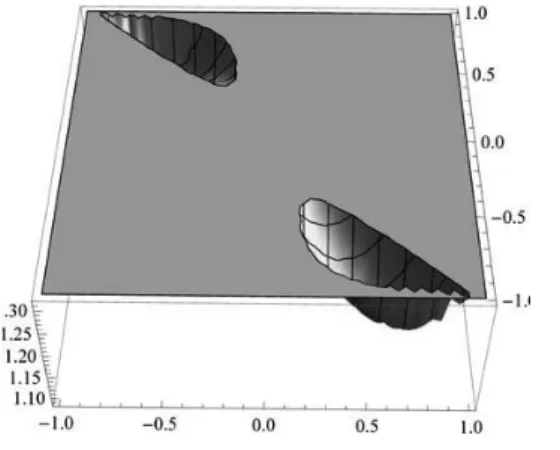
If we fit the ARMA(1,1) model to a special MA(2) process, the function S11x, y has two locally minimal

points. For an example of the MA(2) process with b1 = 0.0, b2 = 0.6, we have the following graph of

S11x, y on the stationary and invertible space of (x, y).

Figure 3. A crosssection of S11x, y with b1 = 0.0, b2 = 0.6.

The problem which we consider is investigating the relation between the parameter of the original MA(2) process and the number of the locally minimal point of the conditional likelihood function S11x, y.

Moreover, it is knowing at what rate it happening.

In order to investigate the minimal point of the function S11x, y, it is first necessary to consider the

admissible parameter space (W2) of MA(2) process with parameters b1 and b2, where

W2 = {(b1,b2); 0§ (b2+b1+1)(b2+b1-1), -2§ b1§ 2, -1§ b2§ 1}. (2.9)

The locally minimal and maximal points satisfy simultaneously the following two equations, ∑S11x, y

∑x

= 0, 2.10

∑S11x, y

∑_y = 0. 2.11

We shall solve the equations as following. The equation (2.10) is equivalent to

x =-y + b1+y2b1-y b12+y b2+y3b2-b1b2-y2b1b2-y b22

1 - 2 y b1+b12-2 y2b2+2 y b1b2+b22. 2.13 Also the equation (2.11) is equivalent to the following equation,

x+ y+ x2_{y+ x y}2_-b 1-x2b1-4 x y b1-y2b1-x2y2b1+x b12+ y b12+x2y b12+x y2b12-x b2-2 y b2-2 x2y b2-4 x y2b2+x y4b2+b1b2+ x2_b 1b2+4 x y b1b2+y2b1b2+x2y2b1b2+x b22+y b22+x2y b22+x y2b22= 0 2.14 From (2.12) and (2.13), we have

-b1-y b2+b1b2 -y b1+b12+y2b12-y b13+b2-2 y2b2+2 y b1b2+3 y3b1b2

-b12b2-4 y2b12b2+y b13b2+2 y4b22-2 y b1b22-3 y3b1b22+b12b22+y2b12b22+b23-2 y2b23+y b1b23 = 0 (2.15)

In general, it is very difficult to solve the equation, but to know the number of the real solutions it is sufficient to consider the resultant of the polynomial

fy = -b1-y b2+b1b2

-y b1+b12+y2b12-y b13+b2-2 y2b2+2 y b1b2+3 y3b1b2-b12b2-4 y2b12b2+y b13b2+2 y4b22-2 y b1b22-3 y3b1b22+

b12b22+y2b12b22+b23-2 y2b23+y b1b23 . 2.16 Since the derivative of the function f(y) is given by

∑ ∑yfy =

b12-2 y b13+b41+6 y b1b2-4 b12b2-12 y2b12b2+12 y b13b2-2 b14b2-b22+6 y2b22-8 y b1b22-20 y3b1b22+5 b12b22+30 y2b12b22

-12 y b13b22+b14b22-10 y4b23+8 y b1b23+20 y3b1b23-4 b12b23-12 y2b12b23+2 y b13b23-b24+6 y2b24-6 y b1b24+b12b24, 2.17

the resultant of the two polynomials (2.16) and (2.17) on y is given as

From the Catastrophe theory, a number of locally minimum points of S11x, y on W2 for MA(2) process

with parameters (b1, b2) is explained by considering a change for the sign of the resultant R(a,b). If the two

polynomials (2.16) and (2.17) have common zeros, the resultant must be vanished. Hence we consider the conditions for R(b1, b2)= 0 on W2. Since the polynomial 1+b12+b222 in (2.18) is always positive on

W₂, it is sufficient to consider the zeros of the polynomial such that

G

1b1, b2 = 1 + b1-b2 -1 + b1+b2 -b1-b2+b1b2 -b1+b2+b1b2  b18+12 b16b2+4 b18b2+48 b14b22+50 b16b22+4 b18b22+64 b12b23+240 b14b23+84 b16b23 -4 b18b23+544 b12b42+357 b14b24+78 b16b42-10 b18b24+512 b25+448 b12b25+636 b14b25+ 64 b16b25-4 b18b52+1632 b12b26+510 b14b62+78 b16b26+4 b18b26+1536 b27+768 b12b27+ 636 b14b27+84 b16b72+4 b18b27+1632 b12b82+357 b14b28+50 b16b28+b18b28+1536 b29+ 448 b12b29+240 b14b29+12 b16b29+544 b21b210+48 b14b210+512 b211+64 b12b211. 2.19 Then we have the following graph for a contour of G1(b1, b2) = 0 on W2.

Figure 4. A contour line of G1(b1, b2) = 0 on W2.

It turns out that the function S11x, y has the two minimum points in a domain (D2) of a portion with a

deep color surrounded with the curve in Figure.5, where

D2= b1, b2 œ W2;1 + b1-b2 -1 + b1+b2 -b1-b2+b1b2 -b1+b2+b1b2 < 0  .

(2.20) Also we define the (bifurcation) set

B2= b1, b2 œ W2; 1 + b1-b2 -1 + b1+b2 -b1-b2+b1b2 -b1+b2+b1b2 = 0 .

(2.21)

When numerical integration is performed by using Mathematica (Ver.7), it turns out that the area of this domain D2 is about 2.490 square, and the rate to the parameter space of a lower triangle is 62.3% exactly.

Figure 5. The domain D2 in W2.

We next determine the property of S11x, y at every point in D2 by considering only one point within

each of the domains.

2.2. Illustrations and Simulation study

2.2.1. Illustrations

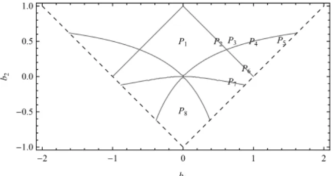
By varying the MA(2) parameters, b1 and b2, continuously and staying inside of D2, for example, going

from position P1 to P2 in Fig.6, the system remains in a stable equilibrium that is the function S11x, y has

two minima. However, if a and b are changed so that the bifurcation set B2 is transversed, something

unusual happens. To see this, start in position P2 of Fig.6, where the system is in a stable equilibrium.

Moving parallel to the b1-axis toward position P3, when the position is reached, the system becomes

unstable the and the function S11x, y has only one minima. There the system is stable again and remains

so while moving onward to position P4. In position P5 inside of D2, it is also seen that the function

S11x, y has two minima.

-2 -1 0 1 2 -1.0 -0.5 0.0 0.5 1.0 b1 b2 P1 P2 P3 P4 P5 P8 P6 P7

Figure 6. Selected MA(2)-parameters (b1, b2) of positions P1- P8.

[1] position P1 ; b1= 0.0 and b2 = 0.5. In this case, S11x, y has two locally minimum points on the

parame-ter space W2 at {x = -0.601501, y = 0.831254} and {x = 0.601501, y = -0.831254} shown in Fig.2.2.1.

[2] position P2 ; b1 = 0.5 and b2 = 0.5. In this case, S11x, y has only one locally minimum on the

[3] position P3 ; b1 = 0.7 and b2 = 0.5. In this case, S11x, y has two locally minimum at {x = 0.896162, y

= -0.907935} and {x = -0.398676, y = 0.90415} shown in Fig.2.2.3.

[4] position P4 ; b1 = 1.0 and b2 = 0.5 (lies in B2). In this case, S11x, y has only one locally minimum at

{x = -0.387582, y = 0.790048} shown in Fig.2.2.4.

[5] position P5 ; b1 = 1.4 and b2 = 0.5. In this case, S11x, y has only one locally minimum on the

parame-ter space W2 at {x = -0.36349, y = 0.675553} shown in Fig.2.2.5.

[6] position P6 ; b1 = 0.9 and b2 = 0.1. In this case, S11x, y has no locally minimum points on the

parame-ter space W2 shown in Fig.2.2.6.

[7] position P7 ; b1 = 0.7 and b2 = -0.085687, which is on the line. In this case, S11x, y has only one

locally minimum points on the parameter space W2 at {x = 0.129372, y = 0.569795} shown in Fig.2.2.7.

[8] position P8; b1 = 0.0 and b2 = -0.5. In this case, S11x, y has two locally minimum at {x = -0.765121,

y = 0.653491} and {x = 0.765121, y = -0.653491} shown in Fig.2.2.8.

The following figures give cross-sectional images of S11x, y with the parameters (b1, b2) of positions

P1- P8, respectively.

　

　　　　　

Figure 2.2.3. S11x, y with b1 = 0.7 and b2 = 0.5. Figure 2.2.4. S11x, y withb1 = 1.0 and b2 = 0.5.

Figure 2.2.5. S11x, y with b1 = 1.4 and b2 = 0.5. Figure 2.2.6. S11x, y with b1 = 0.9 and b2 = 0.1.

Figure 2.2.7. S11x, y with b1 = 0.7 and b2 = -0.08. Figure 2.2.8. S11x, y with b1 = 0.0 and b2 = -0.5.

2.2.2. Computer simulation

We generate a time series of length n = 40,000 from the MA(2) models which are discussed above (1), ... , (8), where the noise is generated from the normal distribution with mean 0 and variance 1. Then we fit an ARMA(1,1) model to each of the time series using the conditional maximum likelihood method with initial values of parameters for the arguments (x, y) of the model. The calculations below are supported by the computer software Mathematica (Ver.7) and an application software ([7]).

0.5 1.0 1.5 2.0 2.5 3.0 f 0.10 0.15 0.20 0.25 0.30 0.35 spectrum

These are plots of the sample auto-correlation function and the sample spectrum. We estimate the ARMA(1,1) model parameters using the conditional maximum likelihood method with some different initial parameter values. The initial parameter values (x = 0.5, y = -0.5) are provided as the arguments of ARMA(1,1) model. Then we have ARMA(1,1) model with {x = 0.604353}, {y = -0.829897} as the conditional maximum likelihood estimate of the model. On the other hand, different initial values (x = -0.5, y = 0.5) lead to another model, ARMA model with {x = -0.598163}, {y = 0.828965}. Therefore we can have two conditional maximum likelihood estimates of an ARMA(1,1) model when we fit the ARMA(1,1) model to the MA(2) process with the parameters (0.0, 0.5), which corresponds to the discus-sion (1) in 2.2.1 and also Figure 2.2.1.

(2) Case when MA(2) process with parameters (b1, b2) = (0.5, 0.5).

0.5 1.0 1.5 2.0 2.5 3.0 f 0.1 0.2 0.3 0.4 spectrum

These are plots of the sample auto-correlation function and the sample spectrum. We estimate the ARMA(1,1) model parameters using the conditional maximum likelihood method with some different initial parameter values. The initial parameter values (x = 0.82, y = -0.86) are provided as the arguments of ARMA(1,1). Then we have an ARMA model with {x = 0.817475}, {y = -0.854429} as the conditional maximum likelihood estimate of an ARMA(1,1) model. On the other hand, different initial values (x = -0.5, y = 0.5) lead to another model, ARMA model with {x = -0.396277}, {y = 0.997437}, this is almost on the boundary of the domain. Therefore we can have only one conditional maximum likelihood estimate of an ARMA(1,1) model when we fit the ARMA(1,1) model to the MA(2) process with the parameters (0.5,0.5), which corresponds to the discussion (2) in 2.2.1 and also Figure 2.2.2.

(3) Case when MA(2) process with parameters (b1, b2) = (0.7, 0.5).

These are plots of the sample auto-correlation function and the sample spectrum. We estimate the ARMA(1,1) model parameters using the conditional maximum likelihood method with some different initial parameter values. The initial parameter values (x = 0.9, y = -0.9) are provided as the arguments of ARMA(1,1). Then we have an ARMA model with {x = 0.883103}, {y = -0.893064} as the conditional maximum likelihood estimate of an ARMA(1,1) model. On the other hand, different initial values (x = -0.5, y = 0.5) lead to another model, ARMA model with {x = -0.393588}, {y = 0.90174}. Therefore we can have two conditional maximum likelihood estimates of an ARMA(1,1) model when we fit the ARMA(1,1) model to the MA(2) process with the parameters (0.7, 0.5), which corresponds to the discus-sion (3) in 2.2.1 and also Figure 2.2.3.

(4) Case when MA(2) process with parameters (b1, b2) = (1.0, 0.5).

0.5 1.0 1.5 2.0 2.5 3.0 f 0.2 0.3 0.4 0.5 spectrum

These are plots of the sample auto-correlation function and the sample spectrum. We estimate the ARMA(1,1) model parameters using the conditional maximum likelihood method with some different initial parameter values. The initial parameter values (x = 0.5, y = -0.5) are provided as the arguments of ARMA(1,1). Then we have an ARMA model with {x = -0.3821}, {y = 0.787593} as the conditional maximum likelihood estimate of an ARMA(1,1) model. On the other hand, different initial values (x = -0.5, y = 0.5) lead to the same model, ARMA model with {x = -0.382131}, {y = 0.787618}. Therefore we can have only one conditional maximum likelihood estimate of an ARMA(1,1) model when we fit the ARMA(1,1) model to the MA(2) process with the parameters (1.0, 0.5), which corresponds to the discus-sion (4) in 2.2.1 and also Figure 2.2.4.

(5) Case when MA(2) process with parameters (b1, b2) = (1.4, 0.5).

0.5 1.0 1.5 2.0 2.5 3.0 f 0.3 0.4 0.5 0.6 0.7 spectrum

(6) Case when MA(2) process with parameters (b1, b2) = (0.9, 0.1). 0.5 1.0 1.5 2.0 2.5 3.0 f 0.1 0.2 0.3 0.4 0.5 spectrum

These are plots of the sample auto-correlation function and the sample spectrum. We estimate the ARMA(1,1) model parameters using the conditional maximum likelihood method with some different initial parameter values. The initial parameter values (x = 0.5, y = -0.5) are provided as the arguments of ARMA(1,1). Then we have an ARMA model with {x = -0.0951825}, {y = 0.994696} as the conditional maximum likelihood estimate of an ARMA(1,1) model, and a different initial value (x = -0.5, y = 0.5) lead to the same model, ARMA model with {x = -0.0951822}, {y = 0.994696}, this is almost on the boundary of the domain. Therefore we have no conditional maximum likelihood estimate of an ARMA(1,1) model when we fit the ARMA(1,1) model to the MA(2) process with the parameters (0.9, 0.1), which corre-sponds to the discussion (6) in 2.2.1 and also Figure 2.2.6.

(7) Case when MA(2) process with parameters (b1, b2) = (0.7, -0.086).

0.5 1.0 1.5 2.0 2.5 3.0 f 0.2 0.3 0.4 0.5 spectrum

These are plots of the sample auto-correlation function and the sample spectrum. We estimate the ARMA(1,1) model parameters using the conditional maximum likelihood method with some different initial parameter values. The initial parameter values (x = 0.5, y = -0.5) are provided as the arguments of ARMA model(1,1). Then we have an ARMA model with {x = 0.134752}, {y = 0.566116} as the condi-tional maximum likelihood estimate of an ARMA(1,1) model. Also, different initial values (x = -0.5, y = 0.5) lead to the same ARMA model with {x = 0.134751}, {y = 0.566117}. Therefore we can have only one conditional maximum likelihood estimate of an ARMA(1,1) model when we fit the ARMA(1,1) model to the MA(2) process with the parameters (0.7, -0.086), which corresponds to the discussion (7) in 2.2.1 and also Figure 2.2.7.

0.5 1.0 1.5 2.0 2.5 3.0 f 0.10 0.15 0.20 0.25 0.30 0.35 spectrum

These are plots of the sample auto-correlation function and the sample spectrum. We estimate the ARMA(1,1) model parameters using the conditional maximum likelihood method with some different initial parameter values. The initial parameter values (x = 0.75, y = -0.65) are provided as the arguments of ARMA(1,1) model. Then we have an ARMA model with {x = 0.766094}, {y = -0.650514} as the condi-tional maximum likelihood estimate of the model. On the other hand, different initial values (x = -0.75, y = 0.65) lead to another ARMA model with {x = -0.774099}, {y = 0.664496}. Therefore we can have two conditional maximum likelihood estimates of an ARMA(1,1) model when we fit the ARMA(1,1) model to the MA(2) process with the parameters (0.0, -0.5), which corresponds to the discussion (8) in 2.2.1 and also Figure 2.2.8.

3. Averaging model of all fitted models

Isn’t there any method of approximating the true model (process) which generated the data

from two or more of the incorrect-identified models? We propose a new method (averaging

model) by use of the estimated ARMA(1,1) models from the example treated in Chapter 2.

The concept for the model averaging is given in bayesian model averaging (Lunn, Jackson,

Best, Thomas and Spiegelhalter [9]). They said that Bernardo and Smith [2] showed

decision-theoretically this provides optimal prediction or estimation under an “M-closed” situation, in

which the true process is among the list of candidate models. Our situation is an “M-open”, in

which the true process is not there any more. In this section we shall only make a suggestion

since the theoretical discussion seems to be very difficult for us.

(1) MA(2) model with b1= 0.0 and b2 = 0.5. In this case, we have two ARMA(1,1) models with

parame-ters {x = -0.601501, y = 0.831254} and {x = 0.601501, y = -0.831254}. The true spectral density function of the MA(2) process and spectral densities of the fitted ARMA(1,1) models are

0.5 1.0 1.5 2.0 2.5 3.0 w 0.10 0.15 0.20 0.25 0.30 0.35 fw 0.5 1.0 1.5 2.0 2.5 3.0 w 0.10 0.15 0.20 fw

Therefore, we define what compounded the spectrum of two applied models (average). It turns out that this reproduces the feature which the original spectrum has. We also define as follows the model which combined two models (average). When the transfer function of the two ARMA(1,1) models is weight averaged, it turns out that this serves as a transfer function of an ARMA(2,2) model. The weight of a weighted average uses the reciprocal of noise variance (in this case, since both two models have equal variance, it serves as an arithmetic average).

1

2 ( 1+0.831254 B1-0.601501 B+ 1-0.831254 B1+0.601501 B) = 1.+0.5 B 2

1.+0. B-0.361803 B2 (3.1)

Thus the averaging model is an ARMA(2,2) model with parameters {0.0, -0.361803} and {0.0, 0.5}.

0.5 1.0 1.5 2.0 2.5 3.0 w 0.10 0.15 0.20 fw 0.5 1.0 1.5 2.0 2.5 3.0 w 0.14 0.16 0.18 0.20 0.22 fw

Spectrum of ARMAmodel[{0.601}, { -0.831}, 1.2] Spectrum of ARMAmodel[{0.0, 0.361803}, {0.0, -0.5}, 1.2]

The averaging spectrum expresses well the feature of the spectrum of a true model (MA(2) process). (2) MA(2) model with b1 = 0.7 and b2 = 0.5. In this case, S11x, y has two locally minimum at {x =

0.896162, y = -0.907935} and {x = -0.398676, y = 0.90415} shown in Fig.3.3.

0.5 1.0 1.5 2.0 2.5 3.0 w 0.1 0.2 0.3 0.4 fw 0.5 1.0 1.5 2.0 2.5 3.0 w 0.1 0.2 0.3 0.4fw

Spectrum of MAmodel[{0.7, 0.5}, 1.0] (True) Spectrum of ARMAmodel[{-0.398}, {0.904}, 1.2]

0.5 1.0 1.5 2.0 2.5 3.0 w 0.21 0.23 0.24 0.25 0.26 0.27 fw 0.5 1.0 1.5 2.0 2.5 3.0 w 0.20 0.25 0.30 fw

The equalization (averaging) spectrum seems to express well the feature of the spectrum of a true model (MA(2) process) rather than the spectrum of the ARMA(1,1) model except for the position of a peak. (3) MA(2) model with b1 = 0.0 and b2 = -0.5. In this case, S11x, y has two locally minimum at {x =

-0.765121, y = 0.653491} and {x = 0.765121, y = -0.653491}. 0.5 1.0 1.5 2.0 2.5 3.0 w 0.10 0.15 0.20 0.25 0.30 0.35 fw 0.5 1.0 1.5 2.0 2.5 3.0 w 0.25 0.30 0.35 0.40 fw

Spectrum of MAmodel[{0.0, -0.5}, 1.0] (True) Spectrum of ARMAmodel[{-0.765}, {0.659}, 1.2]

0.5 1.0 1.5 2.0 2.5 3.0 w 0.25 0.30 0.35 0.40 fw 0.5 1.0 1.5 2.0 2.5 3.0 w 0.20 0.22 0.24 0.26 0.28fw

Spectrum of ARMAmodel[{0.765}, {-0.659}, 1.2] Spectrum of Averaging Spectrum

We can say that the equalization (averaging) spectrum expresses well the feature of the spectrum of a true MA(2) process rather than each spectrum of the ARMA(1,1) models.

4. On misspecified MA(2) model fitting to an AR(2) process

When the incorrect-identified model is applied, how many the misspecified models are presumed? Although the ARMA(1,1) model had been considered until now, even when a true model was which of AR(2) and MA(2), the model obtained with the conditional maximum likelihood method was at most two. It is imagined that the number of the models presumed changes by the model to fit and also by the true process. Here we shall pay attention to MA(2) model. Furthermore, we assume that the time series applied to the model follows AR(2) process. Since calculation is very complicated and generalities are not made, we consider a special case only. These contents serve as extension of the paper before fitting MA(1) model to AR(2) process. We note saying to how many the model which locally maximizes a conditional likelihood function appears. Although it was a maximum of two until now in the case of this MA(2) model fitting, the example in which three models appear is found. And we can confirm the fact in simulation with the case of a large sample.

We consider the case when an MA(2) model is fitted incorrectly to an AR(2) process {X(t)}, (1 - a1B - a2B2) X(t) = e(t). We set the MA(2) model parameters (x, y). In this case, Sp,qQ can be

S

2

x, y = S

2

x, y ; a

1

, a

2



=

_gfx,y_x,y

,

where fx, y = 1- y- x a1-x y a1+y a12-y2a12+a2-x2a2-y a2-x2y a2+

x a1a2-x y2a1a2-y a12a2+y2a12a2-x2a22-x2y a22-y2a22+y3a22+x y a1a22+x y2a1a22-y2a23+y3a23, gx, y = 1  x  y 1  y 1  x  y 1  a2

1  a1 a2 1  a1 a2 1  x a1 y a12 x2a2 2 y a2 x y a1a2 y2a22.

(4.1)

Fallowing to the previous section, we have tried to analysis the locally minimum points of the S2(x, y).

But it is very difficult to solve the general equations such that

∑S2x, y ∑x =0, 4.2 ∑S2x, y ∑y =0. 4.3

Here we present a special example in which the function S2(x, y) has three locally minimal points on the

invertible parameter space. We have the following graph of a crosssection of the S2(x, y) if the fitted model

is an AR(2) process whose parameters are a1 = 0.0 and a2 = 0.95.

Figure 4.1. A crosssection of S2x, y when a1 = 0.0 and a2 = 0.95.

In order to investigate the minimal point of the function S2x, y, it is first necessary to consider its locally

minimal points on the admissible parameter space (W2 A) of AR(2) process with parameters a1 and a2,

where

1.8 x  3.8 x3_{1.805 x}5_{5.79 x y  3.8 x}3_{y  1.805 x}5_{y } 3.99 x y2_{3.4295 x}3_y2_{3.249 x y}3_{3.4295 x}3_y3_{5.04949 x y}4_{1.80049 x y}5 _{ 0} (4.5) 1.9  3.805 x2_{1.71 x}4_{2.19 y  3.8 x}2_{y  5.415 x}4_{y } 5.30525 y2_{7.5905 x}2_y2_{5.14425 x}4_y2_{5.9705 y}3_{6.4885 x}2_y3_{1.6245 x}4_y3_ 4.9495 y4_{3.78599 x}2_y4_{5.41049 y}5_{3.4295 x}2_y5_{1.54327 y}6_{1.62901 y}7 _0 (4.6)

The real solutions of two equations above are shown in Figure.4.2

-1.0 -0.5 0.5 1.0

-1.0 -0.5 0.5 1.0

Figure. 4.2. Real solutions Figure. 4.3. Three locally minimal points We can see in Figure.4.3 that there are three locally minimal points in the domain W2 A such that

A: {0.0, 0.805225}, B: { -1.3453, -0.546645}, C: { 1.3453, -0.546645}.

Corresponding to these points, we have three MA(2) models which have the points for their parameter. We show three spectral density functions of these models and that of the true model.

0.5 1.0 1.5 2.0 2.5 3.0 w 0.5 1.0 1.5 2.0 fw 0.5 1.0 1.5 2.0 2.5 3.0 w 2 4 6 8 fw

Figure.4.4. Spectral density function for A. Figure.4.5. Spectral density function for B.

0.5 1.0 1.5 2.0 2.5 3.0 w 2 4 6 8 fw 0.5 1.0 1.5 2.0 2.5 3.0 w 10 20 30 40 50 60 fw

Furthermore, in the case of a1 = 0.0 and a2 ¥ 0.94, we can also determine that there are three MA(2)

models which are fitted to the AR(2) process.

5. Conclusion

In Section 2, we have considered the misspecified ARMA(1,1) model fitting to MA(2) processes follow-ing to the previous paper[11] in 2012. The conditions for MA(2) parameters on which ARMA(1,1) quasi-likelihood function has more than one local maximum points in the stationary and invertible parameter space were given as the domain D2 for MA(2) parameters (b1, b2) shown in Figure.5. It related to critical

point theory and the behavior of degenerate critical points of the function of two variables in Catastrophe theory, considering the ARMA(1,1) quasi-likelihood function as a potential function with two external parameters b1 and b2.

In Section 4, we have also considered on the misspecified MA(2) model fitting to AR(2) processes. It was already given the domain for AR(2) parameters on which the MA(1) quasi-likelihood function has more than one local maximum point. Our new result presented here is that the MA(2) quasi-likelihood function has three local maximum points in the invertible parameter space W2. Furthermore we have

shown that more general ARMA model has more than three local maximum points in the stationary and invertible parameter space W2. However, I have not performed yet determining the domain where three

models exist in parameter space W2. We will wait for future research findings about this problem.

More-over, is the number of a misspecified model estimated to at most three? We have discovered an example to which six models are estimated by the initial value in a simulation for an ARMA(3,3) model fitting to ARMA(3,6) processes. However, though regrettable, theoretical proof is not made to this result. It is also a future subject about this problem.

Considering these researches, we shall also conjecture that an ARMA(p,q) model has more than one locally maximum points in the stationary and invertible parameter space, if it fitted to a series belongs to an ARMA(p, q+r) process for any positive integer p, q and some r¥1.

The purpose of our research at the last is to investigate what kind of phenomenon happens, when the misspecified model is applied to a certain time series, but probably, it may be insufficient. It will be neces-sary to utilize well two or more models obtained there, and to make it useful for the estimation of a true model, as we discussed in Section 3.

References

[2] Bernardo, J. M. and Smith, A.F.M., 1994, Bayesian theory, John Wiley & Sons, New York.

[3] Box, G.E.P. and Jenkins, G.M., 1970, Time Series Analysis, Forecasting and Control. San Francisco: Holden-Day.

[4] Brockwell, P.J. and Davis, R.A., 1991, Time Series : Theory and Methods, Springer, New York. [5] Castrigiano, D.P.L. and Hayes, S.A., 2004, Catastrophe theory, Westview Press.

[6] Huzii, M., 1988, "Some properties of conditional quasi-likelihood functions for time series model fitting", Journal of Time Series Analysis, 9, 345-352.

[7] He,Y., 1995, Time Series Pack for Mathematica, Wolfram Research.

[8] Kabaila, P., 1983, "Parameter values of ARMA models minimizing the one-step-ahead prediction error when the true system is not in the model set", J. Appl . Prob., 20, 405-408.

[9] Lunn, D., Jackson, C., Best, N., Thomas, A., and Spiegelhalter, D., 2013, The BUGS Book, CRC Press, Boca Raton, FL.

[10] Poston,T. and Stewart, I.N., 1978, Catastrophe theory and its applications, Pitman Publishing Limited.

[11] Tanaka, M., 2012, "On Some Properties of ARMA(1,1) Model Fitting to AR(2) Processes", Bulletin of the Institute of Information Science, Vol.20, 1 - 15.

[12] Tanaka, M. and Aoki, K., 1991, "On a moving average time series model fitting" (in Japanese), Bulletin of the Institute of Information Science, Vol.12, 42 - 54.