Bifurcation structure of stationary solutions of a Lotka-Volterra competition model with diffusion (Mathematical models and dynamics of functional equations)

135

Bifurcation structure

of stationary

solutions

of

a

Lotka-Volterra competition

model with

diffusion

Yukio Kan-On

Department

of

Mathematics, Faculty of Education

Ehime University, Matsuyama, 790-8577, Japan kanon@ed.ehime-u.$\mathrm{a}\mathrm{c}$.Jp

In order to understand the mechanism ofphenomena in variousfields,

we

oftendiscuss theexistence andstabilityof stationary solutionsfor thesystem

ofreaction-diffusion equations

$1_{\mathrm{w}_{x}=0,x=0,1}^{\mathrm{w}_{t}=\epsilon^{2}D\mathrm{w}_{xx}+\mathrm{f}}(\mathrm{w})t’>0x\in(0,1)$

, $t>0,$

(1)

with suitable initialcondition, where $\mathrm{w}\in \mathrm{R}^{N}$,

$\epsilon$ $>0$, $D$ is a diagonalmatrix whose elements

are

positive, and $\mathrm{f}:\mathrm{R}^{N}arrow \mathrm{R}^{N}$ is smooth function.

When $N=1$ is satisfied, we

can

comparatively easily study the existence

of stationary

solutions

for (1) and their spatial profile by the analysis of

motions inthephase plane, becausethe sO-called comparisonprincipleholds.

Furthermore it is well-known that for suitable $f(w)$, the global attractor $A$

of (1) is represented

as

$A= \bigcup_{\epsilon\in E}W^{u}(e)$, where $E$ is the set of stationary

solutions for (1), and $W^{u}(e)$ is

an

unstable manifold of (1) at $w=e$ (for

example,

see

Hale [2, Chapter 4]$)$

.

This fact

means

that

one

of important

problems is to seek all stationary solutions of (1).

In general, the comparison principle does not always hold for the

case

$N\geq 2,$

so

we

have the considerable complexity for studying the existence

and stability of stationary solutions for (1). In this report, as

a

first step to

approach the problem for $N\geq 2,$

we

treat the stationary problem

$\{\begin{array}{l}0=\epsilon^{2}d_{w}w’’+(\mathrm{l}-w^{n}-cz^{n})w0=\epsilon^{2}d_{z}z’,+(1-bw^{n}-z^{n})z,x\in(0,1)w’=0,z,=0,x=0,1\end{array}$ (2)

of

a

Lotka-Volterracompetitionmodel whichismostsimplewithinthe

ffame-woth of

reaction-diffusion

equations, where $’= \frac{d}{dx}$, and every parameter is

a

positive constant.

As

$\mathrm{w}$

means

the population density for two competing

species,

we

restrict

our

discussion topositivesolutions whichsatisfy$w(x)>0$

and $z(x)>0$ for any $x\in[0,1]$

.

It is obvious that (2) has

constant

solutions $(0, 0)$, $(0, 1)$, $(1, 0)$, and $\hat{\mathrm{w}}=$ (u),$\hat{z})$ with

$\hat{w}=\sqrt[n]{\frac{1-c}{1-bc}}$, $\hat{z}=\sqrt[n]{\frac{1-b}{1-bc}}$

136

which is positive for $\max(b, c)<1$

or

$\min(b_{7}c)>1.$ Furthermore the

max-imum principle leads to the fact that every solution of (2) with $w(x)\geq 0$

and $\mathrm{z}\{\mathrm{x}$) $\geq 0$ for any $x\in[0,1]$ must be

a

constant function in _$x$, when

$\min(b, c)<1$ is satisfied.

Let

us

consider the

case

$\mu=(b, c)\in$ $\mathrm{A}/\mathrm{f}$ $\equiv\{(b, c)|\min(b, c)>1\}$.

After

simple calculations,

we see

that for

any

$\mathrm{d}\in$ Vo(ji),

the linearized

operator

of

(2)

around

$\mathrm{w}=\hat{\mathrm{w}}$ has only

one

eigenvalue and at least two

eigenvalues in the right half-plane for any $\epsilon$

with

$\epsilon$ $>1$ and $0<\epsilon<1,$

respectively, where $R_{+}=$ $(0, +\mathrm{o}\mathrm{o})$, $\mathrm{d}=(d_{w}, d_{z})$, and

Vo(ji) $=$

{

$\mathrm{d}\in R_{+}^{2}|\det(-\pi^{2}D+$ fu(w)) $=0$

}.

Thebifurcation theory says that nonconstant positive solutions of (2) which

look like $\pm \mathrm{v}$

case

$x>$ perturbations from $\mathrm{w}=\hat{\mathrm{w}}$ bifurcate at $\epsilon$ $=1$ for any

$\mathrm{d}\in$ Vo(ji), where$\mathrm{v}$ is

an

eigenvectorofthe linearized operatorcorresponding

tothe eigenvalue 0. As themulti-existence ofnonconstant positive solutions

for (2)

is

suggested,

we

shall in thisreport establish the bifurcation structure

ofpositive solutions for (2) with respect to $\epsilon$ forarbitrarilyfixed $\mu\in \mathcal{M}$ and

$\mathrm{d}\in D_{0}(\mu)$

.

Let

us

prepare definitions and notations to state the main result of this

report. We define the order relation $\preceq$ by

$(w_{1}, z_{1})\preceq(w_{2}, z_{2})\Leftrightarrow w_{1}\leq$ $<l\mathit{1}2$, $z_{1}\geq z_{2}$,

anddenote by $\prec$ the relationobtained from the above definition byreplacing

$<$ with $<$. Weset

$\rho=(\mu, \mathrm{d})$, $\mathrm{V}$

$=\cup\{\mu\}\mathrm{x}\mu\in \mathcal{M}$

$D_{0}(\mu)$, $E_{0}(\rho)=R_{+}$ $\mathrm{x}$ $\{\hat{\mathrm{w}}\}$,

$X=$

{

$\mathrm{w}(.)\in C^{2}([0,1])|$w’(0) $=0=$ w(x)}.

For each $\rho\in N,$

we

denote by $\mathrm{E}(\mathrm{p})$ the set of $(\mathrm{e}, \mathrm{w}(.))\in R_{+}\mathrm{x}X$ such

that $\mathrm{w}(x)$ is

a

positivesolution of (2)

for

$\epsilon$, and by $E_{k}(\rho)(k\in \mathrm{N})$ the set of

$(\epsilon, \mathrm{w}(.))\in$

E{p)

suchthat there exists_{$\ell\in\{0,1\}$} such that $(-1)^{j+\ell}\mathrm{w}’(x)\succ 0$

is satisfied

for any $j\in \mathrm{Z}$ and $x\in$ (j/fc,$(j+1)/k$). By definition,

we

see

that

$\bigcup_{k\geq 0}$ Ek$(\mathrm{p})\subset E(\rho)$holds for any $\rho\in N$

,

and that for any $\rho\in II$and $k\in$ N,

$(\epsilon, \mathrm{w}(.))$ $\in$ Ek(p) is equivalent to $(k \epsilon, \mathrm{w}(./k))$ $\in$ E(p).

Theorem 1. $E( \rho)=\bigcup_{k\geq 0}E_{k}(\rho)$ is

satisfied

for

any $n\geq 1$ and$\rho\in N.$

The above theorem says that for each $n\geq 1$ and $\rho\in N,$

we

can

137

structure of$E_{1}(\rho)$. While the structure of Ei(p)

was

completely established

for the

case

$n=1$ in the previous paper [3], the following is for the case

$n>2:$

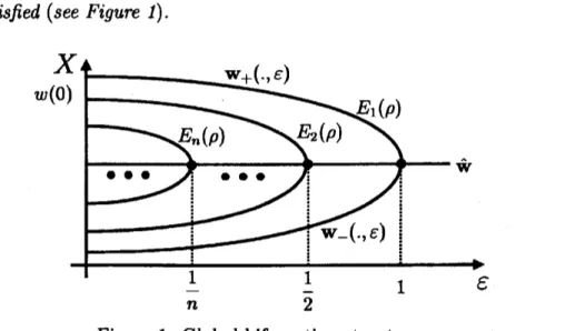
Theorem 2. For each $n\geq 2$ and $\rho\in N,$ there exist continuous

functions

$\mathrm{w}$-(., g) and $\mathrm{w}_{+}($.,$\epsilon)$

defined

on

$(0, 1)$

such that

(i) $E_{1}(\rho)=\{(\epsilon,\mathrm{w}_{\pm}(.,\epsilon))|\epsilon\in (0, 1)\}$,

(ii) 1$\mathrm{w}_{\pm}’(x, \epsilon)\prec 0$

for

any _$x\in$ $(0,1)$ and $\epsilon$

:

$(0, 1)$,

and

(iii) $\lim_{\epsilonarrow}1$Wg$($.,$\epsilon)=\hat{\mathrm{w}}$.

are

_satisfied

(see Figure 1).

Figure 1. Global bifurcation structure.

In consideration of Chafee and Infante [1],

we

see

that the bifurcation

structure of positive solutions for (2) with respect to $\mathrm{e}$ for arbitrarily fixed

$n\geq 2$ and $\rho\in N$ is similarto that for

$\{$

$0=\epsilon^{2}u’’+u(1-u)(u-a)$, $x\in(0,1)$,

$u’(0)=0,$ $u’(1)=0,$

where $0<a<1.$ Furthermore it follows from Kishimoto and Weinberger [4]

that $\mathrm{w}_{-}($.,$\epsilon)$ and $\mathrm{w}_{+}(., \epsilon)$

are

unstable

statio.n

ary solutions for (1).

Figure 2 (a)

and

(b)

are

numerical

bifurcation

diagrams

of

$E_{1}(\rho)$ for the

case

where the assumption of Theorem 2 is violated, and show that the

structure of $E_{1}(\rho)$ depends

on

the interspecific competition rates $b$ and $c$ in

138

$\sim_{\backslash \sim}$ . $\backslash$ 00 $-0^{\cdot}7^{\cdot}$ 0

.,

, , (a) $b=c=$

200.0

(b) $b=c=$

2000.0

Figure 2. Bifurcation structure, where $n=1.1$ and $d_{w}=d_{z}$

.

In the proof of Theorem 2,

one

of important parts is to determine the

geometrical position of the

curve

of positive solutions for (2) bifurcatingfrom

$\mathrm{w}=\hat{\mathrm{w}}$ at $\epsilon=1.$ In general, as the equation which describes the geometrical

position is very complex

even

if

we

can

explicitly write down it,

we

have

difficulty in analyzing the geometrical position theoretically. In theproof, to

determine the geometrical position,

we

employ the numerical verification by

the help

of

the interval

arithmetic

built into Mathematica.

References

[1] N.Chafee and E. F. Infante, A

_bifurcation

problem

_for

a

nonlinearpartial

differential

equation

_of

parabolic type, Applicable Anal. 4 (1974/75),

pp.

17-37.

[2] J. K. Hale, “Asymptotic behavior of dissipative systems”,

American

Mathematical

Society, Providence, $\mathrm{R}\mathrm{I}$,

1988.

[3] Y. Kan-On,

Global

_bifurcation

structure

_of

positive stationary

solutions

for

a

classical

Lotka-

Volterra competition model with diffusion, Japan

J.

Indust.

Appl. Math. 20 (2003), pp.

285-310.

[4] K. Kishimoto and H. F. Weinberger, The spatial homogeneity

_of

sta-$ble$ equilibria

of

some

reaction-diffusion

systems

on convex

domain, J.