土壌の物理性第

(1)

土壌の物理性第一一七号土壌物理学会二〇一一年三月

(2)

土壌の物理性

第 117 ^号 2011 ^年 3 ^月

巻頭言

笹川英夫 . . . 1

論文

Effect of gaps around a TDR probe on water content measurement : Experimental veriﬁcation of analytical and numerical solutions

Toshihiro SAKAKI . . . 3

土壌凍結深や地温が融雪水の下方浸透に与える影響

岩田幸良·長谷川周一·鈴木伸治·根本学·廣田知良 . . . 11

資料

第52回土壌物理学会シンポジウム総合討論

猪迫耕二 . . . 23

土粒子

学生時代を振り返って

森本聡 . . . 31

会務報告

. . . 33

編集後記

. . . 35

表紙写真の説明

花崗岩にTDRのロッドを２本設置して、実験終了後に花崗岩を半分に切断し隙間の有無を調べたところ.今号掲載の論文「Effect of gaps around a TDR probe on water content measurement: Experimental veriﬁcation of analytical and numerical solutions」をご参照ください.

(3)

第 8 ^回（ 2010 年度）土壌物理学会（論文賞）選考結果

土壌物理学会学会賞選考委員会委員長筑紫二郎

学会賞選考委員会として下記論文を論文賞としてふさわしいと決定しました．

1 ．森本聡（ＤＯＷＡエコシステム（株））

永田修（北海道農業研究センター）

川本健（埼玉大学大学院工学研究科）

長谷川周一（北海道大学大学院農学研究科）

2. 対象論文

泥炭林土壌の温室効果ガスの生成と消失，土壌の物理性，第 113 号， pp. 3 ∼ 12 ， 2009 年

3. 推薦理由

陸域面積の 3 % を占める泥炭は全土壌の 1/3 に相当する炭素を含有しているといわれている．

近年，その炭素含有量の多さから，湿地における温室効果ガスの発生が大きく注目されるようになっており，様々な研究が展開されている．しかし，既往の研究の多くは農耕地化された土壌での研究であり，不飽和帯を有する泥炭林や湿地林の土壌が温室効果ガスの給源 / ^{放出源のどちら} に機能するかについて研究した事例は少ない．本研究は，そのような泥炭林土壌における温室効果ガスの挙動を原位置でかつ長期にわたり調査している．表層のみならず，土壌を含む泥炭林における 3 種の温室効果ガスの動態ならびに収支に関する貴重なデータが得られており，今後の地球温暖化研究に大きく貢献するものである．

以上の理由により，本論文を土壌物理学会賞（論文賞）にふさわしいと判断した．

本結果は 2010 年 10 月 23 日に開催された評議員会ならびに総会にて全会一致で承認され，同日授

賞式が開催されました．

(4)

第 8 ^回（ 2010 年度）土壌物理学会賞（ポスター賞）受賞者

土壌物理学会学会賞選考委員会委員長筑紫二郎

開催日： 2010 年 10 月 23 日

会場： 2010 年度土壌物理学会シンポジウム · ^{ポスターセッション}

ポスターセッション参加者の投票ならびに学会賞選考委員会の最終選考により，下記の 5 氏が受賞されました．おめでとうございます．

西脇淳子（明治大学研究 · 知財戦略機構）

ライシメータでの水管理による水稲生育，および温室効果ガスフラックスへの影響

落合博之（明治大学研究 · ^{知財戦略機構）}

深海における TDR 法を用いたメタンバブル発生堆積物中のガス体積の測定

田川堅太（佐賀大学大学院農学研究科）

大型多線式 TDR プローブを用いた面的な表層土壌水分量 · ^{電気伝導度の計測}

柳井洋介（（独）農業 · 食品産業技術総合研究機構，日本学術振興会）

凍結融解土壌における土壌中 N

₂

O 濃度の変化と表層土壌のガス拡散性猪迫耕二（鳥取大学農学部）

土壌カラム実験による表層吸引溶脱法の除塩性能の評価

(5)

会誌「土壌の物理性」の図表作成について（再々）

土壌物理学会編集委員長

会員の皆様には，日頃より学会の運営ならびに会誌「土壌の物理性」へのご投稿，誠にありがとうございます．

学会誌の A4 版 Tex 化による編集に移行してから 2 年が経過いたしました . 皆様のご協力もあって編集作業は円滑に進むようになりましたが，図表の作成に関してはまだ十分とは言えません．

そこで， Tex 化による編集作業をさらに効率的に進めるにあたり，図表の作成に関しまして，現行の原稿執筆要領に加えて，下記の点にご留意いただきますようお願い申し上げます．

○図に関して

· 図は原則としてそのまま組製版されるので，鮮明なものを提出する．

· 図は印刷サイズ（カラム幅 80 mm またはページ幅 170 mm ）で作成する．

· 図中の全ての「線」は 1 pt 以上とする（ hairline は使わない）．

· 図中のフォントは，大きすぎず，小さすぎないサイズとし，全ての図でサイズを概ね統一する．

なお，本文は 10 pt ，図の説明は 9 pt で組版されます．

· 図中のフォントは，日本語については標準的なゴシック系フォントとする．英数字については Arial ， Helvetica ， Symbol ，あるいは Times 系フォントのみとする（ Helvetica の使用を推奨する）．

· 可能な場合，最終原稿の図は EPS 形式で提出する．

○表に関して

· 縦罫線は原則として用いない．

· 最終原稿の表はワープロソフトあるいは MS-Excel などの表計算ソフトで作成し，図としては貼り込まない．

· 表は，印刷サイズ（カラム幅 80 mm またはページ幅 170 mm ）で製版される．ページサイズを超える大きな表は避けること．

現在，原稿執筆要領の改訂を準備しつつありますが，もう暫く時間がかかりそうです．そこで，

上記のようなご協力をお願いする次第です．

会員皆様のご理解とご協力を宜しくお願い申し上げます．

(6)

4 ^月 1 日から原稿投稿先が変わります

現在の学会事務局の任期終了に伴い， 4 月 1 日から編集委員会事務局の場所が変わり，原稿の投稿先が下記のように変更になります。

〒 069-1395 北海道夕張郡長沼町東 6 線北 15 号

（地独）北海道立総合研究機構中央農業試験場内土壌物理学会編集委員会編集委員長中辻敏朗

4 ^月 1 日から土壌物理学会事務局の連絡先が変わります

現在の学会事務局の任期終了に伴い， 4 月 1 日からそのメンバーが替わります．それに伴い，土壌物理学会事務局の連絡先が下記のように変更になります．

〒 060-8589 札幌市北区北 9 条西 9 丁目

北海道大学大学院農学研究院土壌保全学研究室庶務幹事柏木淳一

Tel. 011-706-3641 Fax 011-706-2494

百見は一触にしかず

笹川英夫

¹

言葉遊びのような表題で恐縮である．なぜ，このような表題になったか，経緯を簡単に述べよう．昨秋日本土壌肥料学会の2010年度大会が北海道大学で開かれた．学会発表の合間を利用して，前々から行ってみたいと思っていた近傍施設を見学に訪れるのが学会参加の1つの楽しみである．今回訪れたのは，ニッカウヰスキー余市蒸溜所であった．創建当時の建物が広大な敷地の中に点在する美しさと，創業者竹鶴政孝のウイスキーにかける思いについて話すガイド嬢の素晴らしい説明に感動して帰ってきた．その夜に，旧友と一献傾ける機会があり，ニッカの蒸留所はまさに「百聞は一見にしかず」だったと話をしたら，すかさず彼から「一見」よりももっとパワフルなのは，「一触」だと教えられた．なるほど，土などはまさに百回見るよりも一度触って，その感触を肌で感じた方がうんと効果的ということである．確かに，幼子は土いじりや砂遊びが大好きである．彼らは無意識に土を触り，肌でそのおもしろさを感じているのであろう．甲子園球児が戦い敗れて，悔し涙を流しながら甲子園の土を集めて持ち帰る姿にわれわれは感動するが，選手にとっては，土に触れ，自らの手で土を集めた行為そのものが，来年に向けての雪辱を期す糧になっていると思われる．

私の主たる研究分野は，共生生物窒素固定である．土壌中に存在する微生物と植物とのインタラクションを研究課題にしている関係で，講義は植物栄養，植物生理·生化学，土壌学まで担当している．土壌学の講義で，三角図による土性区分を説明する時に，必ず思い出して学生に話すことがある．40年近く前のことだが，私が大学院生だった時に，静岡大学農学部の加藤芳朗先生の集中講義を聴く機会があった．講義が終わって，大学校内の土を見に行くことになったので私も参加した．晩秋の冷雨が降る中を，親指と人差し指，中指で土をちょっとつまみ，これは埴壌土で粘土は何%，砂が何%と1時間以上もかけて，“指で触れる教育”をしていただいた．先生には申し訳ないが，教室での講義の中味はほとんど記憶にない．しかし，“指で触れる教育”で体験させていただいた土の感触は今でも忘れないでいる．

触って覚えるという行為は何も土に限ったことではない．昨年末，秋田県田沢湖だけに生息し，約70年前に絶滅したとされる淡水魚クニマスが富士五湖の西湖で見つかった．本物であることを確認した京都大学総合博物館の中坊徹次先生は，「魚の見分け方は，本で勉強するより実物の魚を“触って”覚えました」とおっしゃっている．車のボディーのなめらかな曲線は，手で触って確認するのが最も確かという話しも聞いたことがある．職人肌の物作りの名人になればなるほど，指先の感覚（触覚）は視覚の何倍も何十倍も確かな感覚となるのだろう．学生実験や実習の指導にも似たようなことが言える．グループで実験·実習をさせると，手を下してやる学生とそうでない学生が必ずできる．学生実験や実習では，個人が実験器具や装置に触れ，自らの感触として実験·実習の全体像を把握させるのが重要と思っている．したがって，私は，可能な限りそのよう実験·実習のプログラムを組むようにしている．

昨今，「食育」という言葉が盛んに使われているが，「食育」とは「食」に関する知識と「食」を選択する力を習得し，健全な食生活を実践することができる人間を育てることである．「土育」という言葉があるかどうかは知らない．

ましてや，「触育」という言葉があるとはとても思えない．しかし，思えば6，7年前に，土（砂と粘土と言うべきか）

を絞りながら丹念に球体を作り上げていくと，ついには表面のどこにも凸凹がない球体ができ，さらに「さら粉」（土に含まれる乾燥した粘土鉱物）を表面にまんべんなくすり込んでいくと，土とは思えない輝きを放つ，「光る泥だんご」ができるというのがあった．あちこちの幼稚園で実践教育として取り入れられ，園児の教育に一役買ったことを覚えておられ方も多かろう．このような教育が，まさに「土育」，「触育」と言えるのではなかろうか．

生命と環境を育む土の重要性については，土壌に関係する学会等で折に触れ啓蒙活動がなされている．また，土壌観察会が企画され，肌で土の魅力や重要性を伝える取り組みもなされている．土との関わりが希薄になる10代，20 代の若者に，ぜひこのような企画に参加してくれることを願いたい．一方，土壌研究にたずさわる側には，魅力ある

「土壌教育」に関する体系作りが求められよう．私はあと1年で退職するが，土に直接触れて土の魅力や重要性を伝えるような「土壌教育」に貢献できる機会があれば，可能な限り関わりたいと思っている．

1岡山大学大学院自然科学研究科（農学系）

(8)

Effect of gaps around a TDR probe on water content measurement:

Experimental veriﬁcation of analytical and numerical solutions

Toshihiro SAKAKI

¹

Abstract: When installing TDR probes to rock, void spaces (gaps) between the probe rods and rock may be en- countered. In this study, the dielectric constants of water and air were measured with various controlled gaps and effects of the gaps were experimentally investigated. We focused on a two-rod probe for which analytical and numerical solutions were available. Symmetric longitudinal gaps (identical uniform gaps along both rods), non-symmetric longitudinal gaps (uniform gaps along only one rod), and end gaps beyond the end of the rods were considered. For the symmetric cases, measured dielectric constant values of water and air were compared with analytical and/or numerically simulated values, and a close agreement was observed. For the non-symmetric cases, such agreement was seen only when the gap width was relatively small. As the gap widths increased, the dielectric constant of water was underestimated compared to the numerically esti- mated values. Such underestimation was more signiﬁcant when the gaps were along the rod connected to the center conductor, suggesting that the sensitivities of the two rods were uneven. The effect of the end gaps was very limited whereas the longitudinal gaps, e.g., due to loose guide holes or soil shrinkage can lead to signiﬁcant measurement errors.

Key Words: water content, dielectric constant, time domain reﬂectometry, gap effects, measurement errors

1. Introduction

After the work by Topp et al. (1980), time domain reﬂec- tometry (TDR) has been widely used since the early 1980’s for soil water content measurement in various problems in soil science, agriculture, environmental and geotechnical applications. The standard device consists of a pulse gen- erator, a probe and a data logger. The method requires the probe to be embedded into the material of interest. The probe is usually made of two or three metal rods connected to a coaxial cable. The transmission velocity of an electromagnetic step pulse along the probe is measured and converted into water content (e.g., Topp et al., 1980).

1Environmental Science and Engineering Division, Colorado School of Mines, Golden, Colorado, U.S.A. Corresponding author: Toshihiro Sakaki

2011年1月27日受稿 2011年3月8日受理土壌の物理性117号, 3–9 (2011)

When applying TDR to rock, guide holes must be drilled prior to the probe installation. Hokett et al. (1992) reported that the probe must be in good contact with rock in order to obtain accurate measurements of moisture content. Even when slightly undersized guide holes are used, it is difﬁcult to eliminate the longitudinal and end gaps around the probe completely, because the guide holes are not drilled with a perfectly-matching diameter, nor are they exactly as long as the probe rods. Sakaki et al. (1998) showed a couple of photographs in which these gaps are clearly visible.

Annan (1977) considered the case of non-concentric gaps, which coincided with a bipolar coordinate system (Morse and Feshbach, 1953) centered at the probe loca- tions, and derived an analytical expression for the apparent dielectric constant (Ka). Knight (1992) analytically showed that the highest measurement sensitivity occurs in the vicinity of the probe rod surface. This implies that if slight void spaces or gaps exist between the rod and the material, the measurement accuracy may be affected. This is especially true if the gaps are filled with material that has a smaller dielectric constant than that of the surrounding medium. Ferré et al. (1996) and Knight et al. (1997) used numerical simulations of the Laplace equation to estimate the influence of gaps on apparent dielectric constant. They showed that for small gaps, the analytical results of Annan (1977) were valid even for concentric gaps. Sakaki et al.

(1998) and Sakaki and Rajaram (2006) presented extensive data on the application of TDR to water content (θ^{) mea-} surement on rocks. The data of Sakaki et al. (1998) were obtained using probes hammered into slightly undersized guide holes. The Ka-θ data could not be explained without invoking the potential role of air-filled gaps around the probe rods, which was eliminated later by filling the gaps with electrically conductive silicone (Sakaki and Rajaram, 2006). Despite the above mentioned works for identifying the effect of gaps, to our best knowledge, the gap effects have never been experimentally “measured” in a quantita- tive fashion under well-controlled conditions, and the analytical and numerical approaches for quantifying the gap effects have never been verified against experimental data.

The objectives of this study were; (1) to experimentally

(9)

4 土壌の物理性第117号 (2011) demonstrate the inﬂuence of gaps on errors in estimates

of Ka under well-controlled conditions, (2) to verify the analytical and numerical solutions for the gap effects and (3) to quantitatively illustrate the magnitude of potential errors in moisture content estimates, resulting from gaps around TDR probe rods in soils/rocks based on analytical/numerical calculations for some practically relevant sit- uations. We considered gaps along the rod surfaces (hereafter referred to as the “longitudinal gaps”) and gaps beyond the end of the rods (hereafter referred to as the “end gaps”). Because the analytical and numerical solutions were available for the longitudinal gaps along a two-rod probe, we focused only on the two-rod probe. The experimental results were compared to theoretical estimates, where available, obtained using the analytical solution as well as numerical solution of the Laplace equation, with speciﬁed potential on the rod surfaces, and incorporating the inﬂuence of longitudinal gaps.

2. Material and methods

We considered uniform longitudinal gaps around the rods and end gaps beyond the end of the rods to mimic the gaps that are expected in the field applications as shown in Fig. 1(a). When fully saturated, the gaps are filled with water whereas the gaps are likely to be filled with air when unsaturated. The typical pore size in the rock matrix is usually smaller than the size of the gaps, causing a larger suction in the matrix. Therefore, water tends to be retained in the matrix due to its larger suction, which consequently makes the gaps fill with air.

Fig. 1 Two-rod TDR probe; (a) Longitudinal and end gaps when installed into rocks, (b) Tested conﬁguration in the experi- ments.

2.1 Probe conﬁguration

The TDR probe used in this study was the two-rod type as shown in Fig. 1(b) and is a practical configuration for application to rocks. A couple of spade tongues were sol- dered to the split end of a 50Ωcoaxial cable (RG58/AU), which were screwed to an acrylic plate having dimensions of 60×100×10 mm. Brass rods with a diameterd= 10 mm, center-to-center spacings=30 mm, and length l=200 mm, were attached to the screws above. The cable was, in turn, connected to a commercially available time domain reflectometer TDR100 (Campbell Scientific, Inc., Logan, Utah). The reflectometer emits an electromagnetic step-pulse with a voltage of 250 mV and a 10∼90 % rise time of 200 picoseconds (frequency spectrum roughly up to 1.75 GHz, Tektronix, Inc.,1987), which is transmitted along the coaxial cable and probe. The TDR traces were processed by software PCTDR (Campbell Scientific, Inc., Logan, Utah) and apparent dielectric constantKawas calculated.

2.2 Longitudinal gaps

2.2.1 Experimental setup for longitudinal gaps In reality, the longitudinal gaps may vary in space as in Fig. 1(a) but those cannot be quantified. Therefore, in the context of quantifying the effects of longitudinal gaps around a TDR probe, we considered equivalent uniform widths. In order to mimic air-filled gaps with thin but uniform thickness in water, polyvinyl chloride (PVC) tape with a uniform thickness was used. The dielectric constant of PVC is substantially smaller than that of water (KPVC= 2.9 81) (e.g., Converting Technology Institute, 1997) thus, its effect is analogous to air-filled gaps in unsaturated rock, which is considered to be the most likely situation in the field. The PVC tape was carefully wound to the rod surface to create uniform-thickness gaps. The PVC gap thicknesses (δ) considered were; 0.0 (no gap), 0.107, 0.160, 0.317, 0.475, 0.636, 0.792 and 0.950 mm. The PVC tape was applied up to 6 layers so that the gap width (thickness of the entire PVC layer) was approximately 1 mm (10

% of the rod diameter), which seemed to be large enough for the investigation of gap effects in a practical sense. The values of gap width were obtained by measuring the diameter of the rod with and without the PVC tape using a digital caliper, taking the difference of the two, and were considered the “actual” thickness of the PVC tapes when the measurements were taken. For each gap width, uniform identical gaps along both rods (hereafter “symmetric cases”) and uniform gaps only along one rod (hereafter “non-symmetric cases”) were considered. The non- symmetric cases were further divided into two categories;

uniform gap along the rod connected to the center conductor (hereafter “center rod” or CT), and uniform gap only

(10)

論文：Effect of gaps around a TDR probe on water content measurement 5 along the rod connected to the shield (hereafter “shield

rod” or SH).

2.2.2 Analytical solution for longitudinal gap ef- fect

Using the bipolar coordinate system (Morse and Fesh- bach, 1953), Annan (1977) ﬁrst derived the analytical solution for the longitudinal gap effect for a two-wire probe with non-concentric gaps around the rods. Based on his solution, the analytical solution for the apparent dielectric constant Ka of water measured by a two-rod probe with non-concentric circular gaps is;

Ka= Kgapξ0

Kmaterial(ξ⁰−ξ¹) +Kgapξ¹^K^material ⁽¹⁾ where,Kgap is the dielectric constant of the gap material, Kmaterial is the true dielectric constant of the material of interest, ξ0andξ1are the radial bipolar coordinates that can be calculated from rod radius, gap width, and the half- distance between bipolar foci (see Annan, 1977 for details).

2.2.3 Numerical solution for longitudinal gap ef- fect

Unfortunately, use of equation (1) is limited to symmetric cases where identical uniform gaps exist along both rods. If the gaps exist only partially, or more generally, if the medium surrounding the probe is heterogeneous, a numerical method must be employed.

Assuming that the TDR probe rods have an inﬁnite length, the electrostatic potential ﬁeld in the plane perpendicular to the rods is described by the Laplace equation.

Knight et al. (1997) showed that the apparent relative dielectric constantKacould be calculated by the following equation.

Ka=

S1

Kgap

∂φ

∂n

ds

S1

∂φ0

∂n

ds

(2)

where,Kgapis the dielectric constant of gap material,φ ^is the electrostatic potential for non-homogeneous case (with gaps), φ0 is the electrostatic potential for homogeneous case (without gaps),nis the outward pointing unit normal vector on the boundary,S1is the internal boundary for a rod.

Knight et al. (1997) showed that concentric gaps completely surrounding both rods could be modeled reasonably accurately using the analytical solution for non-concentric gaps. Thus, in this study, “concentric” gaps were deﬁned in the ﬁnite element mesh around the rods of a two-rod probe. The dimensions of the domain were approximately 20sin thex-direction and 12sin they-direction, where swas the center-to-center rod separation that was 30 mm

in this case. The diameter of both rods wasd =10 mm.

A no-ﬂux boundary was imposed on the outer boundary (S3) on the domain. The nodes on one rod (S1) were set to a constant potential of−1, the potentials on the other rod (S2) were set to 1 (see Knight et al., 1997 for details).

PVC-filled gaps were incorporated by assigning KPVC= 2.9 to appropriate elements whereasKwater=81 was given to all the other elements. The finite element mesh was con- structed so that the thickness of the gaps could be varied from 0.01 mm to 10 mm. To confirm the accuracy of the model, the symmetric cases were computed first and the results were compared to the analytical solution. Then, the non-symmetric cases were simulated. It should be noted that in the numerical simulation, both rods were identical and the possible uneven contribution between the center and shield conductors was not taken into account in the model.

2.3 Experimental setup for end gaps

For the investigation of the end gap effect, a solid PVC rod was used to establish gaps at the end of rods. A cylin- drical piece of PVC rod with a diameter equal to the rod diameter of 10 mm sliced to have a pre-speciﬁed length was directly glued to the end face of each rod. The thickness of the glue was kept as thin as possible so that its effect was minimized. Since PVC has a dielectric constant of 2.9, it should act like air when measured in water. The end gap lengths considered were; 0, 1, 1.5, 2, 3, 4, 5, 7.5, 10, 15 and 20 mm.

3. Results and discussion

3.1 Effect of longitudinal gaps

Fig. 2 shows the experimental, analytical, and numerical results of the dielectric constant of water with the longitudinal PVC gaps. For each gap thickness, five measurements were taken and averaged. In the analytical and numerical calculations, Kwater =81 was used (von Hippel, 1995). For the symmetric cases, the experimental results (large solid circles) agreed closely with the analytical and numerical results. As can be intuitively inferred, the larger the gap widthsδ, the larger their effects. In this case, since Kgap<Kwater, the dielectric constant of water was more underestimated asδ increased. For comparison, the effects of “air”-filled gaps were also calculated using equation (1) and shown in Fig. 2 by a gray solid line. It caused more underestimation than PVC-filled gaps. This was expected because the dielectric constant of air was less than that of PVC. For the typical gap width range of 0.1 ∼0.3 mm (Sakaki et al., 1998), PVC-filled and air-filled gaps caused up to 46 % and 71 % underestimation in theKavalues, re- spectively, when measured in water with the probe configuration tested. In this study, a relatively large rod diameter was used so that we were able to investigate gap effects for

(11)

6 土壌の物理性第117号 (2011)

Fig. 2 Effect of PVC- ﬁlled gaps in water (d=10 mm,s=30 mm). The thick solid line denotes the analytical dielectric constant calculated using equation (1) when gaps are ﬁlled with PVC (KPVC=2.9). The dashed lines are the results from numerical simulation and equation (2) for the symmetric and non-symmetric cases. Data for the no gap are plotted atδ=0.001 mm. Note that the uneven contribution between the CT and SH rods was not taken into account in the numerical model.

Fig. 3 Effect of PVC-ﬁlled gap in air (d=10 mm,s=30 mm).

The solid line denotes the analytical dielectric constant calculated using equation (1) when gaps are ﬁlled with PVC (KPVC=2.9).

The result for the no gap case is plotted at gap=0.001 mm.

smallδ/d ratios. However, it must be noted that equation (1) implies that for a probe with a smaller rod diameter, the underestimation will be even more signiﬁcant.

For the non-symmetric cases, theKavalues were closer to 81 than those obtained for the symmetric cases. This observation was expected because only one rod had the gaps, thus, the effect was less. Two SH cases withδ =0.107 and 0.160 mm on the shield rod, whereδ was small and within the typical range, agreed well with the numerical results. In other SH cases withδ =0.317∼0.950 mm on the shield rod, the experimental results tend to show lower Kavalues than numerical results. All CT cases with gaps on the center rod showed smallerKa values than those in the SH cases.

Fig. 3 shows the results for PVC-ﬁlled gaps measured in air (gaps on both rods only). The analytical values

calculated by equation (1) are denoted by a solid line.

Although the measured dielectric constant values were slightly higher than the analytical values, their behavior was well explained by equation (1). For the typical gap width of 0.1∼0.3 mm as Sakaki et al. (1998) observed, the overestimation of the dielectric constant in air due to the PVC-ﬁlled gaps was up to 2 % and not as signiﬁcant as the 46 % underestimation observed in water.

3.2 Effect of end gaps

The results for the end gap effects are plotted in Fig. 4.

As there are no analytical and numerical solutions available for this case, only experimental results are presented.

For each end gap length, ten measurements were taken.

The effects were relatively small compared to those for the longitudinal gaps presented in the previous section. The obtainedKavalues were normalized by 81 so that the end gap effects were seen in terms of relative errors. Baker and Lascano (1989) reported that sensitivity ends abruptly at the end of the probe, i.e., changes in water content just beyond the end of the rods have no effect on the signal. Our data showed that the presence of void space filled with air caused a slight underestimation of the apparent dielectric constant and that the effect was almost constant regardless the size of the void space. For an infinite transmission line, the electromagnetic pulse transmits in the sim- plest mode referred to as TEM (transverse electromagnetic wave), where the electric filed, magnetic field, and direction of propagation are perpendicular to each other (Kraus, 1991). Near the end of rods, the wave is transmitted in higher modes, which has possibly been affected by the presence of air and caused the slight underestimation of the dielectric constant. This is probably limited to a very small region at the end of the rods and thus the effect is as much as∼2 % regardless the size of the void space. Al- though the results are probably unique for the probe dimensions shown here, it is recommended that the void length be minimized as much as possible.

Fig. 4 Normalized dielectric constant of water measured with various end gap lengths.

(12)

論文：Effect of gaps around a TDR probe on water content measurement 7

Fig. 5 Calculated water content and relative error with water- and air-ﬁlled gaps in a hypothetical rock with true water content of 0.1 (squares), 0.25 (triangles), and 0.4 (circles). Probe dimensions;d=10 mm,s=30 mm.

3.3 Gap effects on water content in soils and rocks

In the previous sections, the gap effects were investigated using limited materials such as water, air, and PVC.

The combination of these materials resulted in somewhat different contrast of dielectric constants than that of our interest, i.e., rock and air-filled gaps, rock and water-filled gaps and so on. Similar relationships for apparent dielectric constant Ka vs. gap width δ were calculated using equation (1) for both air- and water-filled gaps in a hypothetical rock material. The dimensions of the two-wire TDR probe were assumed to be d=5 mm, s=30 mm which are typical for commercially available probes (d= 2.4∼4.8 mm,s=14∼40 mm, TRIME system, IMKO, Inc., Ettlingen, Germany; d=3.2∼4.8 mm, s=30∼ 45 mm, Campbell scientific, Inc., Logan, Utah;d=3 mm, s=12.5∼37.5 mm, TRASE system, Soilmoisture Equip- ment Co., Santa Barbara, California). For demonstration purposes, it was assumed that Topp’s equation (Topp et al., 1980) to relateKaandθwas valid for the hypothetical rock material.

The apparent dielectric constantKaof the rock (includ- ing air and water phases) was assumed to be 5.9, 13.4, and 25 that correspond to water content of 0.1, 0.25 and 0.4 using Topp’s equation. For the probe conﬁguration mentioned above, the apparent dielectric constant was computed using equation (1), and converted into water content.

The calculated water content as well as relative errors are plotted in Fig. 5.

4. Discussion and conclusions

The effects of longitudinal and end gaps were experimentally investigated and, where available, the results were compared to the analytical and numerical solutions.

Although the end gaps showed very little effects, the longitudinal gaps lead to signiﬁcant errors. For the symmetric longitudinal gaps, where uniform identical longitudinal gaps were on both rods, the experimentally measured data

showed good agreement with the analytical and numerical solutions. For the non-symmetric cases, where the longitudinal gaps exist along one rod only, the results were not as straightforward. The cases with gaps on the center rod showed more effect than those with gaps on the shield rod. When an electromagnetic step pulse propagates along a coaxial transmission line, the center conductor carries the signal and the shield conductor is ground; i.e., “unbalanced” signal. In a transmission line consisting of two parallel conductors, both conductors carry a signal, equal in magnitude but opposite in sign with the ground potential in the center plane; this is referred to as “balanced”

with respect to ground. For a two-rod TDR probe, the electrical ﬁeld will gradually change from unbalanced to balanced (without using a balanced-unbalanced transformer, e.g., Spaans and Baker, 1993), which often leads to higher sensitivity on the rod connected to the center conductor.

The uneven contribution of each rod leads to a difference in the trace data depending on whether the gaps are on the CT or the SH rod as shown in Fig. 6. If the balanced electrical ﬁeld cannot be obtained within the length of the probe, the

Fig. 6 Example traces withδ=0.636 mm obtained in water.

Longitudinal gaps are on CT rod only, SH rod only, and both rods.

Trace with no gap is also shown for comparison.

(13)

8 土壌の物理性第117号 (2011) CT rod will carry more signal than the SH rod. Therefore,

when measured in water, the gap effect is expected to be more distinct when PVC-filled gaps are present along the CT rod, which resulted in more underestimation inKain this case. The trace with gaps on the CT rod shows two reflections; one from the CT rod, and another from the SH rod without gaps that indeed corresponds to the reflection point of the no gap case. For the trace with gaps on the SH rod, the second reflection disappeared. Overall, the experimental data revealed that the analytical and numerical solutions were valid to quantify the effect of symmetric longitudinal gaps. Because of the uneven contribution of the rods, the numerical solution tends to somewhat un- derestimate the effects when the longitudinal gaps are not symmetric.

When applying TDR to unsaturated rocks, it is likely that the gaps are filled with air rather than with water due to larger suction in the surrounding matrix. Thus, the results imply that much attention should be paid to minimize gaps around the probe rods when applying TDR to rocks, as air-filled gaps are the potential cause for significant underestimation ofKa values of the rocks, thus, water content. An electrically conductive material may be used to fill such gaps to minimize their effects on the measurement accuracy (Sakaki and Rajaram, 2006). Moreover, gaps can arise not only for rocks but also for soils if sufficient care is not taken when packing soil around the probes (Decagon Devices, 2010), if the sensor is dislocated inside the soil, or when soil shrinkage occurs. Therefore, maximum attention has to be paid to ensure good contact between the probe and the material of interest when installing probes in soils or rocks.

We have experimentally shown that the center rod is more sensitive than the shield rod. Limsuwat et al. (2009) showed similar non-symmetric characteristics in the commercially available capacitance sensors. Even when there is no gap, the non-symmetric characteristics can lead to some implications. For example, if a probe is aligned such that the rods experience a large water content difference between the two, the measurement may be biased. When measuring a wetting front migration and one of the rods is in the wet region and the other is in the dry region, the resultingKais likely to be affected more when the center rod is in the dry region.

Acknowledgements

This research was partially supported by Japan Nuclear Cycle Development Institute (JNC Cooperative Research Scheme on the Nuclear Fuel Cycle).

References

Annan, A.P. (1977): Time domain reﬂectometry — Air-gap prob- lem for parallel wire transmission lines. Report of Activities,

Part B, Pap. 77-1B, pp. 59–62, Geol. Surv. of Canada, Ottawa, Ont. Canada.

Baker, J.M. and Lascano, R.J. (1989): The spatial sensitivity of time domain reﬂectometry. Soil Science, 147: 378–384.

Converting Technology Institute (1997): The material guidebook for converting 1997/98. pp. 333–334, (in Japanese).

Decagon Devices Inc. (2010): Why does my soil moisture sensor read negative? Decagon Devices Virtual Seminar Series.

Ferr´e, P.A., Rudolf, D.L. and Kachanoski, R.G. (1996): Spatial averaging of water content by time domain reﬂectometry: Im- plications for twin rod probes with and without dielectric coatings. Water Resour. Res., 32: 271–279.

Hokett, S.L., Chapman, J.B. and Russell, C.E. (1992): Potential use of time domain reﬂectometry for measuring water content in rock. J. Hydrol., 138: 89–96.

Knight, J.H. (1992): Sensitivity of time domain reﬂectometry measurements to lateral variations in soil water content. Water Resour. Res., 28: 2345–2352.

Knight, J.H., Ferr´e, P.A., Rudolph, D.L., Kachanoski, R.G.

(1997): A numerical analysis of the effects of coatings and gaps upon relative dielectric permittivity measurement with time domain reﬂectometry. Water Resour. Res., 33: 1455–

1460.

Kraus, J.D. (1991): Electromagnetics : Fourth edition. p. 850, McGraw-Hill, New York.

Limsuwat, A., Sakaki, T. and Illangasekare, T.H. (2009): Ex- perimental quantiﬁcation of bulk sampling volume of ECH₂O soil moisture sensors. Proceedings of the 29th Annual Ameri- can Geophysical Union Hydrology Days, March 25–27, 2009, ed. J.A. Ramirez, pp. 39–45, Colorado State University, Fort Collins, CO.

Morse, P.M. and Feshbach, H. (1953): Methods of theoretical physics. Part II, McGraw-Hill, New York.

Sakaki, T., Sugihara, K., Adachi, T., Nishida, K. and Lin, W.R.

(1998): Application of time domain reﬂectometry to determination of volumetric water content in rock. Water Resour. Res., 34: 2623–2631.

Sakaki, T. and Rajaram, H. (2006): Performance of different types of time domain reﬂectometry probes for water content measurement in partially saturated rocks. Water Resour. Res., 42, W07404, doi:10.1029/2005WR004643.

Spaans, E.J.A. and Baker, J.M. (1993): Simple balun in parallel probes for time domain reﬂectometry. Soil Sci. Soc. Am. J., 57: 668–673.

Topp, G.C., Davis, J.L. and Annan, A.P. (1980): Electromagnetic determination of soil water content: Measurements in coaxial transmission lines. Water Resour. Res., 16: 574–582.

Tektronix, Inc. (1987): Tektronix metallic TDR’s for cable testing, Application Note. pp. 1–16, Beaverton, Oregon.

von Hippel, A. (Ed.) (1995): Dielectric Materials and Applica- tions. p. 438, Artec House, Norwood, Mass.

(14)

論文：Effect of gaps around a TDR probe on water content measurement 9

要旨

TDRプローブを岩石に設置する際にはプローブと岩石試料との間に隙間が発生することがある．本研究では，既知の隙間を持つプローブを用いて水と空気の比誘電率を計測し隙間の影響を評価した．隙間の影響に関する理論解および数値解が存在する2ロッド型プローブについて，両ロッドに対称に隙間がある場合，片方のロッドのみに隙間がある場合，そしてロッド先端以深に隙間がある場合について検討した．対称な隙間のケースでは，水と空気の比誘電率の計測値は理論解および数値解とよく一致した．

非対称のケースでは隙間幅が比較的小さい場合は数値解と一致したが，隙間幅が大きくなるとともに実験結果の方が数値解より大きな影響を示した．実験結果および数値解の差異は隙間が同軸ケーブルの芯線に接続したロッドにある場合により顕著に見られ，ロッド間で感度が異なることがわかった．ロッド先端部以深の隙間の影響は小さかったが，ガイド孔が緩い場合やプローブ周辺の土壌で乾燥収縮が発生するような場合には含水率が過小評価される可能性があることが示された．

キーワード：含水率,比誘電率,時間領域反射率法,隙間の影響,計測誤差

(15)

土壌凍結深や地温が融雪水の下方浸透に与える影響

岩田幸良

¹

· ^{長谷川周一}

²

· ^鈴木伸治

³

· ^根本学

⁴

· ^廣田知良

⁴

Effects of soil frost depth and soil temperature on downward soil water movement during snowmelt period

Yukiyoshi IWATA¹，Shuichi HASEGAWA²，Shinji SUZUKI³，Manabu NEMOTO⁴and Tomoyoshi HIROTA⁴

Abstract: Frozen soil layer sometimes impedes the snowmelt infiltration into deep soil layer, which decreases the amount of soil water recharge and delay the transporta- tion of nitric acid to deep soil layer. To investigate the relationship between soil frost and snowmelt infiltration, three years field observation was conducted at the arable field located in Tokachi region in northernmost island of Japan.

Two plots were prepared and snow on the one plot was re- moved for approximately one month to enhance the soil freezing. As a result, soil frost depths at the beginning of snowmelt period were ranged between 0.1 and 0.5 m. The amount of infiltrated water into below 0.5 m depth during snowmelt period was calculated from the field data. The strong relationship between the frost depth and the ratio of snowmelt infiltration to the available snowmelt water (infiltration ratio) was obtained, whereas there were no clear relationships between the infiltration ratio and soil temperature at 0.05 m depth just before the beginning of snowmelt period. Thus, the frost depth is one of the most important factors to estimate the amount of snowmelt infiltration into deep soil layer when the frost depth is relatively shallow.

We explained the process of the decrease in the snowmelt inﬁltration with the increase in the soil frost depth using a conceptual model.

Key Words : frozen soil layer, snow cover, soil water movement, inﬁltration ratio, snow-removal treatment

1. はじめに

土壌は凍結すると透水係数が低下する（e.g., Miller, 1980; Watanabe and Flury, 2008）．そのため，融雪期に凍結層が存在すると融雪水の浸透が抑制され，表面流出量が増加することで，土壌侵食（Øygarden, 2003）や河川の流量の増加（Shanley and Chalmers，1999；鵜木ら，

1National Agricultural Research Center for Hokkaido Region, NARO;

Sinsei, Memuro, Kasai-gun, Hokkaido, 082-0081, Japan. Corresponding

author:岩田幸良，（独）農研機構北海道農業研究センター

2Field Science Center for Northern Biosphere Hokkaido University; Kita 11 Nishi 10, Kita-ku, Sapporo, Hokkaido, 060-0811, Japan.

3Department of Bioproduction and Environment Engineering, Tokyo University of Agriculture; 1-1-1 Sakuragaoka, Setagaya, Tokyo, 156- 8502, Japan.

4National Agricultural Research Center for Hokkaido Region, NARO;

Hitsujigaoka 1, Toyohira-ku, Sapporo, Hokkaido, 062-8555, Japan.

2010年5月12日受稿 2011年3月23日受理土壌の物理性117号, 11–21 (2011)

2003）を引き起こす場合がある．融雪水の土壌への浸透により，土壌中の硝酸態窒素も下層に移動する（西尾ら，

1988；Derby and Knighton，2001）．そのため，北海道のように積雪水量の多い地域では，春の施肥設計や，耕地の表層から地下水への硝酸態窒素の移動量を評価する上で，融雪水の下方浸透量の適切な評価が必要とされる．

最大土壌凍結深が0.5 m以上になる北米や北欧では，

融雪期における土壌凍結層の水分量や地温が，融雪水の浸透量の多少に大きな影響を与えることが指摘されている（Granger et al., 1984; St¨ahli et al., 1996; Zhao et al., 1997）．一方，最大土壌凍結深，もしくは融雪期直前の土壌凍結深が浅い地域では，ほとんど全ての融雪水が土壌中に浸透したという報告例がある（Iwata et al., 2008）．

Komarov and Makarova（1973）も，凍結層中の氷の量のほか，土壌凍結深が浅くなることで融雪水の浸透量が増加することを指摘している．しかし，土壌凍結深が比較的浅い地域で土壌への融雪水の浸透量を評価した事例は少ない．

筆者らは，冬の降水量が300 mm程度と世界的にみると比較的多雪な北海道の十勝地域に観測サイトを設置し，土壌水分量の観測や深さ0.50 mの水フラックスの推定をおこなった．同地域では，1990年代前半までは，年によって最大土壌凍結深が0.4 mよりも深くなった．しかし，現在は多量の降雪により，土壌が冷たい空気から断熱される時期が早期化したことで，深さ0.2 m程度までしか土壌が凍結しなくなった（Hirota et al., 2006）．そこで，自然積雪条件の試験区（対照区）のほか，除雪をすることで土壌凍結を発達させる試験区（除雪区）を設置し，2005年11月から2006年4月まで観測を実施した．その結果，対照区と除雪区の土壌凍結深はそれぞれ

0.1, 0.4 m程度になり，対照区ではほとんど全ての融雪水

が融雪期に土壌に浸透したのに対し，除雪区では融雪期において土壌水の下方浸透が抑制されたことを報告した

（Iwata et al., 2010a）．このように，土壌凍結深が極端に異なる場合には，融雪期における下方浸透量が大きく異なる可能性がある．しかし，土壌凍結深と融雪水の下方浸透量の関係を定量的に評価した研究はほとんど無い．

融雪期には冬の間に地表面に堆積した降水が短期間に地表面に供給されるため，最大土壌凍結深の浅い近年の十勝地域では融雪期に最も土壌水分量が多くなり

(16)

12 土壌の物理性第117号 (2011)

（Hirota et al., 2009），一年で最も土壌水の下方浸透が卓越することが知られている（Iwata et al., 2010b）．そこで本研究では，同観測サイトにおいて上記の期間を含む3 年間の長期観測を行い，融雪期直前の土壌凍結深が0.11

∼0.52 mの範囲にあるときの融雪期の下層（0.50 m以

深）への土壌水の浸透量を定量的に評価した．本研究の目的は，融雪期直前の土壌凍結深や融雪期以前の地温と，

融雪期における下方浸透量との関係を評価し，土壌凍結深が深くなることで融雪水の浸透が抑制されるメカニズムを提示することにある．

2. 材料と方法

2.1試験圃場と観測項目

北海道十勝地域の中部に位置する北海道農業研究センター芽室研究拠点の試験圃場（42^◦53’ N，143^◦05’ E）に観測サイトを設置した．観測圃場から約5 km西に位置する気象庁の観測地点（アメダス芽室）で1979∼2000 年に観測された1月と7月の平均気温は，それぞれ−9

◦Cと18^◦Cである（気象庁，2010）．また，同観測地点において1979∼2000年に観測された12∼2月の積算降水量と年降水量の平均値は，それぞれ117 mmと969 mm，1月の最大積雪深の平均値は0.61 mである（気象庁，2010）．試験圃場は台地上に位置し，土壌は淡色黒ボク土である（農耕地土壌分類委員会，1995）．地下水位は8ｍ程度と低く（岡，2000），深さ1 mまでの土層の飽和透水係数は10⁻⁴∼10⁻⁶m s⁻¹と高い．

試験圃場に5ｍ×5ｍの2つの試験区を1 mの間隔をおいて設置した．除雪区では約1ヶ月間の除雪処理を行い，土壌凍結を促進させた．目標とする凍結深に到達してから，除雪を終了した．試験圃場の土層構造や各土層の基本的物理性，試験区のレイアウトの詳細については Iwata et al.（2010a）を参照されたい．観測期間は2005 年11月から2008年4月である．2005∼06年には目標とする土壌凍結深（0.4 m）に到達してから除雪区に雪を被せ，積雪深が対照区と同じになるようにした．それ以外の年については，雪を被せる作業は行わなかった．対照区では積雪に対する処理を行わなかった．試験期間中は，除草剤により植生がない状態で地表面を管理した．

計測機器設置のため，各試験区のほぼ中央に深さ1.5 mの試坑を掘った．深さ0.05 mから1.05 mまで，0.1 m 間隔でロッド長0.3 mのTDRプローブ（CS605, Camp- bell社）を鉛直断面に水平方向に挿入し，TDR水分計

（TDR100, Campbell社）により土壌水分量のプロファイ

ルを測定した．各土層から撹乱土を採取し，TDR水分計で計測される比誘電率を体積含水率に換算する多項式を求めた．この試験の際，TDR水分計の影響範囲が直径

80 mmの範囲内に納まっていること，温度変化による

TDRの出力値の変化（Wraith and Or, 1999）は無視できるほど小さいことを確認した．なお，TDRで計測される凍土の液状水量は，凍結前の水分量の影響を受ける場合があることが報告されているが（Suzuki, 2004; Watanabe

and Wake, 2009），今回の観測では，土壌が凍結する直前

の深さ0.05 mの土壌水分量に極端な差がみられなかっ

たことから（3.1節参照），この影響を無視しても問題ないと考えた．土壌水分計の他，除雪区は深さ0.40 mまで，対照区は深さ0.20 mまでの土層に0.02∼0.05 m間隔で熱電対を埋設し，これらの土層より下の層には0.10 m間隔で熱電対を埋設し，深さ1.00 mまでの地温プロファイルを測定した．これらのセンサーを設置後，試坑を丁寧に埋め戻した．測定深さの間の地温を線形補完により推定し，0^◦C以下の深さを凍土と仮定して土壌凍結深を計算した（融雪期後期の対照区では，表層の地温がほぼ0^◦Cの期間が数日間続く年があったが，このときも地温が0^◦Cの土壌は凍結していると判断した）．水分計·地温計を埋設した地点から2 m程度離れた試験区内の地点に深さ1.5 mの試坑を掘り，深さ0.90 mと1.00 mにテンシオメータを埋設した．埋設したテンシオメータは，断熱材と小さな熱源を用いて計測機器内の脱気水の凍結を防止し，土壌凍結条件でも凍結層より下の非凍結土壌の圧力水頭を長期間計測できる特徴をもつ（Iwata and Hirota, 2005a, b）．また，高さ1.20 mに超音波積雪

深計（SR-50, Campbell社）を設置した．これらのデー

タは10秒間隔でサンプリングし，10分間隔でデータロ

ガー（CR23X, Campbell社）に記録した．他の観測要素

よりも計測に時間を要する土壌水分量については，独立したデータロガー（CR1000, Campbell社）により，10 分間隔で計測したデータを記録した．

気温は，試験圃場から100 m程度離れた気象観測露場において，高さ1.90 mに設置した通風筒の中の温度

計（HMP45A, Vaisala社）により計測した．降水量は，

同露場において高さ1.40 mに設置した，雪の捕捉率を上げるためのフェンス（RT-4）がついた溢水式降水量計

（B071-20，横河電機）により測定した．これらのデータ

もデータロガー（CR10X, Campbell社）に10分間隔で記録した．冬期の降水が雪であるか雨であるかを目視により判断した．

1週間に2度，定規で積雪深を測定し，超音波積雪深計の値を補正した．このとき，スノーサンプラーにより積雪水量も測定した．試験圃場では，雪面からの蒸発量は通常，0.5 mm d⁻¹未満であり（Hayashi et al., 2005），

融雪期の積雪水量の減少（1∼15 mm d⁻¹）に比べて少なかった．そこで，雪面蒸発による積雪水量の減少は無視できると仮定し，計測された積雪水量の減少量と降水量から融雪水量を計算した（岩田ら，2010）．

2.2融雪期の下方浸透量の評価

試験圃場は平坦な地形のため，深さ1.00 mまでの土層の水の流れを鉛直一次元のみと仮定し，水収支の計算により融雪期の下方浸透量を推定した．ダルシーの法則を不飽和まで拡張した以下のリチャーズ式により深さ0.95 mの水フラックス（q0.95; m s⁻¹)を計算した．

q0.95=−k(ψ0.95)×(ψ0.90−ψ1.00+L)/L (1) ここに，k(ψ0.95)^は深さ0.95 mの圧力水頭（ψ0.95（m））

(17)

論文：土壌凍結深や地温が融雪水の下方浸透に与える影響 13 に対する同深さの不飽和透水係数（m s⁻¹），ψ0.90とψ1.00

はそれぞれ深さ0.90 mと1.00 mの圧力水頭（m），L^は圧力水頭測定地点間の距離（=0.10 m）である．土壌水が鉛直上向きに移動する時，q0.95は正の値をとる．深さ

0.95 mを含む土層（3C層）から，直径113 mm，高さ

50 mmの円筒試料を採取した．この試料を実験室に持

ち帰り，圧力水頭（ψ^{）が高いとき（}⁰≥ψ≥ −1.40 m）には定常法により（Hasegawa and Sakayori, 2000），定常法では精度の高い測定が難しかった圧力水頭が低いとき（−1.40 m>ψ^{）には非定常法（}^{One Step}^法^{; Doering,} 1965）により，不飽和透水試験を行った．実験により得られた不飽和透水係数と圧力水頭の関係を次式で近似した（Iwata et al., 2010a）．

log(k(ψ)) =−3.93|ψ|³+13.3|ψ|²−14.9|ψ| −3.63 (0 m≥ψ≥ −1.40 m)

=1.62×10⁻⁴|ψ|⁶−7.50×10⁻³|ψ|⁵ +0.121|ψ|⁴−0.935|ψ|³+3.74|ψ|²

−7.46|ψ| −4.44 (ψ<−1.40 m)

(2) ψ⁰.90とψ¹.00の平均値として計算したψ0.95と，式（2）から，各水分状態における透水係数を計算した．融雪期には，融雪水の浸透により土壌が湿潤化するため，

ヒステリシスの影響が大きいと考えられる高水分領域

（0≥ψ≥ −1.40 m）の近似式は，定常法による湿潤過程の透水試験により求めた．

灌漑計画を立てる際の有効土層が地表面から深さ0.50

∼0.60 mまでの土層とされることから（駒村，1992），消

雪後に深さ0∼0.50 mに含まれる水や窒素肥料は作物に有効に利用される可能性が高いと考えられる．また，

本試験で採用したTDR土壌水分計による凍土中の水分量の測定値は，土壌の全体積に対する液状水の割合に相当し，凍土中の氷の量は反映されない．そのため，観測データから土壌水分移動量を水収支法で評価する際には，氷の融解や液状水の凍結による水分計の出力値の増減が誤差要因になる．そこで，本論文では，観測期間中に土壌が凍結しなかった0.50 m以深を対象とした，次の水収支式により，深さ0.50 mにおける融雪期の水フラックス（q0.50; m s⁻¹）を計算した．

q0.50=q0.95−ΔS0.50−0.90/Δt (3) ここに，ΔS0.50−0.95 は単位時間（Δt; ここでは1 日=

86400 s）におけるTDR水分計の出力値から計算される

深さ0.50∼0.95 mの水分貯留量の増加量（m）である．

計算されたq0.50 を積分し，符号を逆転させて（すなわち，鉛直下向きの水移動を正として），融雪期に深さ0.50 mを浸透した水の量（INF0.50; mm）を計算した．なお，

本論文では，1日の融雪水量が1 mm以上になり，かつそ

の後に3日間以上の連続的な融雪が認められた日から消雪日の前日までを融雪期とした．強風による雪の再分配で試験区内の積雪水量が減少することが1∼2月にあったため，雪の再分配の有無を目視で確認し，融雪期間の判定を誤らないようにした．融雪期には雪の再分配は確認されなかった．

土壌凍結層により融雪水の浸透が多少抑制されても，

融雪期間が長期化し融雪水量が多ければ，INF0.50の値が大きくなると考えられる．また，深さ0∼0.50 mの土層中の水分量が少ないほど，融雪水はこの土層の水分量を増加させるために使用され，0.50 m以深への浸透に寄与しない融雪水の量が増加すると考えられる．そこで，これらの影響を考慮した以下の式により，融雪期における相対的な浸透割合（IR）を評価した．

IR=INF0.50/(ΣM−ΔSSW) (4) ここに，ΣMは融雪水量（mm），ΔSSWは深さ0∼0.50 mの水分貯留量が少なかった年に，同土層の土壌水分量の増加に使われ，0.50 m以深には浸透しない融雪水量

（mm）である．ΔSSWの計算には，次の二つの時期にお

ける深さ0∼0.50 mの水分貯留量を用いた：①土壌凍結

層が融雪水の浸透を抑制せず，十分な融雪水が土壌に浸透した年の，消雪日の前日の水分貯留量（Sb）；②各年の各試験区における融雪期直前の水分貯留量（Sx）．土壌凍結層が存在しなくても，消雪日の前日には深さ0∼0.50 mの水分貯留量がSbになる．そこで，SxがSbよりも小さい場合は，凍結層が存在しなくても両者の差分だけ融雪水が土壌水分量の増加に使用され，0.50 m以深には浸透しないと考え，次式によりΔSSWを計算した．

ΔSSW=Sb−Sx (5) 試験圃場では，融雪期直前の土壌凍結深が0.10 m程度であれば，融雪水のほとんどが土壌に浸透することが知られている（Iwata et al., 2008, 2010a, b）．2005∼06年の対照区の融雪期直前の土壌凍結深は0.11 mであり，かつ融雪水量は90 mmであった（3章参照）．そこで，この年の対照区の消雪日直前の深さ0∼0.50 mの水分貯留量をSbとした．この年の消雪日直前にはまだ土壌凍結層が残っており，土壌水分量の測定深さのうちで最も

浅い0.05 m深の土壌は凍結していたと考えられる．こ

の深さのTDR水分計が氷の量を評価できないことでSb が過小評価されることを避けるため，次の融雪期における水収支式によりSbを計算した．

Sb=S2006CO+ΣM2006CO−INF0.50−2006CO (6) ここに，S2006CO，ΣM2006CO，INF0.50−2006COはそれぞれ 2005∼06年の融雪期直前の深さ0∼0.50 mの水分貯留量（mm），融雪期の総融雪水量（mm），融雪期の深さ

0.50 mにおける総下方浸透量（mm）である．

(18)

14 土壌の物理性第117号 (2011)

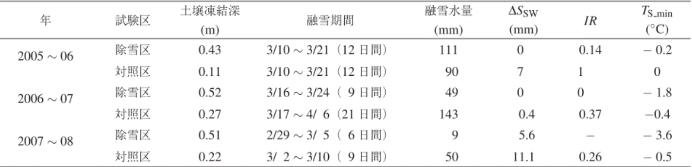
Table 1 各冬の各処理区における最大土壌凍結深·融雪期間·融雪水量．表中のΔSSWは，深さ0∼0.50 mの土層の水分量が少

ない年に，深さ0.50 m以深に浸透する水分量が減少することを考慮するための補正値である（詳細は本文参照）．式（4）により計算される融雪水の浸透割合（IR）と融雪期直前に計測された地温プロファイルの最低値（TS min）も表中に示した．2006∼07 年の除雪区の浸透割合は，融雪水量が極端に少なかったために計算の対象からはずした．

Annual maximum soil frost depth, snowmelt period, amount of snowmelt during snowmelt period, inﬁltration ratio calculated form Eq. (4) (IR), and lowest soil temperature at the beginning of snowmelt period (TS min).ΔSSWis snowmelt water not to inﬁltrate below 0.50-m depth, which is caused by the dry soil condition to the depth of 0.50 m (see text for detail). The data at the treatment plot in the winter of 2006 – 07 was not calculated due to the very small amount of snowmelt water.

年試験区土壌凍結深

(m) ^融雪期間

融雪水量 (mm)

ΔSSW

(mm) IR TS min

(^◦C)

2005∼06 ^除雪区 0.43 3/10∼3/21（12日間） 111 0 0.14 −0.2

対照区 0.11 3/10∼3/21（12日間） 90 7 1 0

2006∼07 ^除雪区 0.52 3/16∼3/24（ 9日間） 49 0 0 −1.8

対照区 0.27 3/17∼4/ 6（21日間） 143 0.4 0.37 −0.4

2007∼08 ^除雪区 0.51 2/29∼3/ 5（ 6日間） 9 5.6 − −3.6

対照区 0.22 3/ 2∼3/10（ 9日間） 50 11.1 0.26 −0.5

式（5）のSxと式（6）のS2006COは，土壌が凍結を開

始してから融雪期の直前までの次の水収支式により計算した．

Sx=Sa+UF (7) ここに，Saは土壌凍結層が形成される直前（初冬）の深さ0∼0.50 mの水分貯留量（mm），UFは土壌凍結層が発達するときに下層から深さ0∼0.50 mの土層に供給される水分量（mm）である．深さ0.05∼0.45 mの土壌水分量の測定値からSaを計算した．UF ^は式（3）により計算される深さ0.50 mの水フラックスを積分して求めた．

なお，2005∼06年の除雪区では，式（5）のΔSSWが

−4 mmであった．これは，融雪期以前に土壌凍結層に多量の水が存在したことを意味している．TDR水分計から計算した融雪期直前の深さ0∼0.50 mの液状水量

（166 mm）は，Sb（240 mm）よりもかなり少なく，過剰な水は氷として存在したことがわかる．ΔSSWの計算で導出された4 mmも氷として存在し，土壌凍結層の融

解と共に0.50 m以深に浸透すると考えられる．しかし，

2005∼06年の除雪区では，消雪日まで土壌凍結層の不凍水量に顕著な変化はみられず，融雪期に土壌凍結層の顕著な融解はなかったと考えられる．そこで，この年の除雪区で氷として存在した過剰水が融雪期に下層に浸透することはなかったと考え，このときのΔSSWを0 mm とした．

3. 結果

3.1積雪深·土壌凍結深·土壌水分量の推移

観測期間の冬期における気温，積雪深，土壌凍結深，深さ0.05 mと0.55 mの土壌水分量（以下，それぞれθ0.05 とθ0.55；土壌が凍結した場合は液状水量を意味する）の

推移をFig. 1に示す．また，冬期の各処理区における

最大土壌凍結深，融雪期の期間，融雪水量をTable 1に

示す．

いずれの年も，11月下旬から12月上旬の間に日平均気温がマイナスになり（Fig. 1a），対照区·除雪区ともに土壌凍結深が増加した（Fig. 1c）．対照区では，12月下旬から1月上旬の間の積雪により積雪深が0.20 mを超え，それ以降は土壌凍結深がほぼ一定で推移した．一方，除雪区では，除雪処理をおこなったことで土壌凍結深がその後も増加した（Fig. 1b, 1c）．その結果，年最大土壌凍結深は対照区で0.11∼0.27 mであったのに対し，

除雪区では0.43∼0.52 mとなり，処理区間で大きな差がみられた（Table 1）．2005∼06年は目標とする土壌

凍結深を0.4 mとし，これに達した後に人工的に雪を被

せて積雪深を対照区と同じにする処理をおこなった．一方，2006∼07年と2007∼08年は，除雪処理後に雪を被せる処理を除雪区で行わなかったため，対照区に比べ除雪区の融雪水量が少なくなった（Table 1）．

土壌凍結層が形成されると，液体の水が凍結することでθ0.05が急激に減少した（Fig. 1d）．下層から凍結層へと水が鉛直上向きに移動したことで（Iwata et al.,

2010a），土壌凍結深が深くなるにつれてθ0.55も減少し

た（Fig. 1e）．除雪処理を行う前までは，両処理区のθ0.55 は同等であった．しかし，深さ0.3 m以上の積雪により対照区で土壌凍結深の増加が停止すると，対照区のθ0.55 は，除雪区よりも緩やかに減少した．対照区では，土壌凍結の発達が止まったことで凍結前線の水ポテンシャルの減少が抑えられ，凍結前線よりも下層の鉛直上向きの水フラックスが減少したと考えられる．一方，除雪区では，除雪処理により土壌凍結深が増加し続けたため，下層から凍結層に向かう水フラックスが減少しなかったと考えられる．その結果，両試験区のθ0.55の差はどの冬も最大で0.05 m³m⁻³程度になった（Fig. 1e）．

2006∼07年には，12月下旬の気温の上昇（Fig. 1aの

①）と12月27日の33.5 mmの降雨により，降雨直後

にθ0.05とθ0.55が増加した（Fig. 1d, 1e）．しかし，その後，土壌凍結深が再び増加すると，θ0.05とθ0.55が急速

土壌の物理性第