Transactions of the JSME (in Japanese)
日本機械学会論文集
セグメントの加減速運動に起因するマシニングセンタの 円弧補間工具経路の誤差推定
丘 華
*1Trajectory error estimation to circular arc interpolation cutter path of machining center
due to acceleration/deceleration motions of interpolation segments Hua QIU
*1*1 Department of Mechanical Engineering, Kyushu Sangyo University 2-3-1Matsukadai, Higashi-ku, Fukuoka 813-8503, Japan
Abstract
From the machining center (MC) user’s point of view, the author proposes a practical approach to estimating the trajectory errors of a circular arc interpolation cutter path produced by the NC servo characteristics for a target MC in this paper. Firstly, a simple and convenient acceleration/deceleration procedure model is given for describing the behavior of the servo axes in an interpolation motion of circular arc segments. This model contains two parameters whose value is necessary to be identified by experiments. The first is the time constant of the servo axes and its value can be easily determined from the radius reduction in circular motion trajectories corresponding to different radius and feed rate. The second is a timing parameter to define the time interval of the acceleration and the deceleration procedures between two interpolation segments, and its value can be readily identified from a measured trajectory of two circular arc cutter path. Based on the model and an assumption, in which the motion of each segment is independently performed, a concise and efficient simulation algorithm to calculate a cutter path trajectory composed of many circular arc segments in detail is developed. Comparison results of the simulated cutter path trajectories with the measured ones and the contours of work pieces machined under the same motion condition sufficiently demonstrate the effectiveness and reliability of the proposed approach. Therefore, as a useful tool, the approach is applicable to beforehand estimating the influence of the NC acceleration/deceleration motions on cutter path accuracy or judging the motion conditions for the machining purpose without performing an actual machining test with the machining center.
Keywords : Machining center, Cutter path, Motion trajectory, Error estimation, Accelepolation/deceleration motion, Circular arc interpolation, Motion error model, Parameter identification, Simulation
1. 緒 言
マシニングセンタ(以下,MC と略す)を使用してワークの輪郭を精密に加工する際に,工具経路を直線補間 または円弧補間により生成することがよくある.この場合,補間セグメントのNC加減速運動により実際の工具 経路に運動誤差が発生し,加工したワークの輪郭には形状誤差が生じる.直線補間工具経路について,NC 加減 速運動に起因するセグメント間の接合部における丸み誤差(コーナ部誤差),ないしそれに対応する多数の短いセ グメントからなる工具経路の運動誤差に関しては詳細に研究されている(Kwon and Burdekin, 1998; Schmitz and Ziegert, 2000; Iwasawa et al., 2004; Shih et al., 2004; 松原,2008; 斎藤他,2012; Otsuki et al., 2019a; 丘他,1998, 2010, 2013).一方,MCの円運動については,NC制御に起因する運動誤差による円運動の半径減少がよく知られてお り(垣野他,1986, 1987; 松原,2008),加工したワークの輪郭精度に影響する円弧補間工具経路の運動誤差を抑 えるために,MC 送り駆動系の加減速設計法や CNC パラメータのチューニング法および工具経路の調整法も提
Received: 1 April 2019; Revised: 20 May 2019; Accepted: 17 June 2019
No.19-00150 [DOI:10.1299/transjsme.19-00150], J-STAGE Advance Publication date : 25 June, 2019
*1 正員,九州産業大学理工学部(〒813-8503 福岡県福岡市東区松香台2-3-1)
E-mail of corresponding author: [email protected]
Qiu, Transactions of the JSME (in Japanese), Vol.85, No.875 (2019)
案されている(山崎他,2000; 鈴木他,2003; Uddin et al., 2007).しかし,多数の円弧補間セグメント,特に短い セグメントからなる工具経路の運動誤差に関する研究が少ない.近年では,工具材料,工作機械,CAD/CAM技 術の進歩によって,精密輪郭切削において,短い補間セグメントからなる工具経路の採用とともに,用いる送り 速度も著しく増加している.そのため,生産現場において工具経路の運動誤差に起因する輪郭誤差によってワー クの加工精度と加工効率の面にトラブルを引き起こす恐れがある(斎藤他,2012; Gassara et al., 2013; 長坂他,
2018).本来,MCのNC装置内部に用いた加減速運動の制御則やサーボ系のパラメータが分かれば,切削をせず
に切削運動パラメータに対応する運動誤差を推定して把握することが可能であるが(松原,2008),通常では,MC の使用者にとってこのようなNC装置内部制御の詳細は開示されていない.例えば,異なるNCシステムの内部 において工具経路の補間処理や加減速制御などについてメーカ各自の手法の利用が考えられるが,それらの詳細 及び加工精度に及ぼす影響は MC の使用者にとってブラックボックス的存在になることもある(Otsuki et al., 2019b).
そこで,本研究では,MCの使用者の立場から,比較的簡単な形で円弧補間運動におけるNC加減速運動モデ ルを立て,簡単なMC工具経路の運動軌跡を測定した結果からモデルに必要なパラメータの値を同定する方法を 提案する.また,この運動モデルに基づき,工具経路の運動軌跡を簡便にシミュレーションするアルゴリズムを 提案する.さらに,工具経路軌跡のシミュレーション結果を,実測したMCの運動軌跡および仕上げたワークの 輪郭誤差と比較することにより,提案した円弧補間運動の加減速運動モデルとパラメータの同定結果,工具経路 運動軌跡シミュレーション方法の妥当性を示す.
2. 円弧補間運動における加減速運動モデル
本研究に使用するMCはワシノ製セミクローズドループ方式のWMC-4立形中型MCである.そのX軸,Y軸,
Z軸の移動範囲はそれぞれ900 mm,450 mm,510 mmである.NCシステムはFANUC Series 0-MBであり,同時 制御軸数は2.5軸,最小設定単位は1mである.テーブルの構造はX軸テーブルがY軸テーブルの上に載せられ た構造であり,Z軸はコラム構造である.最大切削送り速度は5000 mm/minである.NCシステムの取扱説明書 によれば,切削送りの加減速運動制御は指数関数形加減速方式が採用されている.また,このNCシステムには NCプログラムのブロック先読み機能がない.
以前に行った直線補間工具経路の運動誤差に関する研究には,対象MCの各駆動軸サーボ系について一次遅れ 特性を持ち,かつ軸間に相互干渉がないように取り扱うことができた(丘他,2010).この結果は,NC工作機械 の駆動軸サーボ系において,電流制御系と速度制御系の交差角周波数(Bandwidth)が位置制御系の交差角周波数 より十分高い場合,位置制御系のクローズドループ伝達関数が一次遅れ系に近似できるという理論解析結果と実 際経験(杉本他,1990)に一致している.
したがって,本研究では,対象MCの各駆動軸の位置サーボ系を一次遅れ系として取り扱い,各軸サーボ系の 入出力関係を図1のブロック線図で定義する(Ogata, 2002).図中のTは位置制御系の時定数(以下,単に駆動軸 サーボ系時定数と略す)であり,Re(s)とOu(s)はs領域で記述するサーボ系の入力(指令値)と出力(応答)で ある.時間領域(t領域)で記述する系の入出力をre(t)とou(t)で記せば,つぎのラプラス-逆ラプラス変換の関 係が成り立つ.
()
1 ) 1
1 ( ) 1
( )
( 1 1 1 ret
s Ts Ts Re
s Ou t
ou
L L L L
(1)2・1 円弧補間運動のパラメータと指令値
図2に円弧補間運動のパラメータを示す.図中のX軸とY軸は運動平面を構成するMCの第1と第2駆動軸で ある.XY平面において,開始点S(Xs, Ys),終了点E(Xe, Ye),中心C(Xc, Yc),半径R(mm),中心角の円弧に そって送り速度F(mm/s,その値は反時計回りの場合に正,時計回りの場合には負とする)を指令して円運動を させるとき,X軸とY軸の経路座標(X, Y)は次の式となる.
Fig. 1 Simplified block diagram of a servo axis.
Fig. 2 Parameters of a circular arc segment.
cos( ) cos
())
cos( t X R t R X X t
R X
X c s s (2)
sin( ) sin
())
sin( t Y R t R Y Y t
R Y
Y c s s (3) 式中のtは時間で,X(t)とY(t)はX軸とY軸サーボ系への変位指令である.なお,は円弧補間運動の公称 角速度, は開始点Sに対応する位相角であり,それらの値は式(4)と(5)による.
R F/
(4)
) ,
( 2
atan YsYc XsXc
(5)
ここで,atan2(y, x)はy/xの逆正接関数で,その値はyとxの符号の組合せにより[0,2]の領域で唯一に決まる.
XとYを時間tについて微分すると,送り速度の指令値Fx,Fyは次の式となる.
) sin(
/d
d
X t F t
Fx (6)
) cos(
/d
d
Y t F t
Fy (7)
2・2 円弧補間運動の指令値に対する MC 駆動軸の出力
MCのX軸とY軸は互いに独立な一次遅れ系であるので,式(2)と式(3)のX(t)とY(t)を入力として式
(1)で示す変換処理を施せば,X軸とY軸の位置出力xとyは次の式のように表すことができる.
x x
sT t x x
x
s T e t X
T X F
t Ts X
x x
1 cos( ) cos( )
) 1 )(
sin(
1 )
1 ( 1
2 2
1
L
L
(8)
y y
sT t y y
y
s T e t Y
T Y F t Ts Y
y y
1 sin( ) sin( )
) 1 )(
cos(
1 )
1 ( 1
2 2
1
L
L
(9)ここで,TxとTyはそれぞれX軸とY軸サーボ系の時定数であり,パラメータxとyは次式のように定義される.
実際のMCのNCシステムにおいてTxとTyが同じ値に設定されていたので,本研究ではTxTy Tとする.そ うすると,
x tan1(Tx )tan1(Ty ) y tan1(T ) (10)
xとyの式は次のような形になる.
sT t
X t
e T
T
x F
1 cos( ) cos( )
) 1 )(
sin(
2 1
2
(11)
Re(s) Ou(s)
1 1
Ts
X Y
O
S E B
C
R F
Qiu, Transactions of the JSME (in Japanese), Vol.85, No.875 (2019)
sT t
X t
e T
T
y F
1 sin( ) sin( )
) 1 )(
cos(
2 1
2
(12)
また,xとyについて時間tで微分すると,X軸とY軸の速度出力vxとvyは次の式のように得られる.
sin( ) sin( )
2 1
2
e t
T
v F T
t
x (13)
cos( ) cos( )
2 1
2
e t
T
v F T
t
y (14)
円弧セグメントの長さが十分であれば,式(11)と(12)に基づいて円弧補間運動軌跡の半径rは次のように 求められる.
2
2 2 21 x X y Y R T
r c c (15) したがって,T221であれば,円弧補間工具経路軌跡の半径減少量rは次式で表される.
R F T r R
r 0.5 2 2/
(16)
2・3 円弧補間セグメントの加速運動時間と減速運動
図2に示した円弧補間運動においては,各駆動軸が0から加速し,時刻t1で指令終点Eより前の点Bから減速 する.t1以後の減速運動における駆動軸の速度出力は次の式のように表される(丘他,2010).
T t t x
x v t e
v
1
) (1
(17)
T t t y
y v t e
v
1
) (1
(18) 式中のvx(t1)とvy(t1)は式(13)と(14)から求める時刻t1での駆動軸出力速度である.点Sから点Bまでの円弧 補間運動の加速時間t1をt1で記せば,その値は指令する円弧補間運動の経路長と送り速度から定まる.
t1R/F (19) なお,付録に示すように,加速運動時間t1に対して点Bからの減速運動が式(17)と(18)に従えば,円弧補間 運動はちょうど指令終点Eに停止することが確認できる.
2・4 前後の円弧補間セグメントの加減速運動タイミング
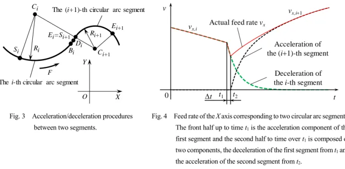
図3にMC工具経路における前後の補間セグメントの加減速運動関係を示す.前のi番目セグメントが時刻t1
に対応する点Biから減速していく.時間tの遅れで次のi+1番目セグメントが時刻t2t1tに対応する点Diか ら加速し始める.このtはNC装置内部の加減速制御やセグメント処理などに係わり,サンプリングタイムと関 連する時間パラメータである(斎藤他, 2012; Saito et al., 2016; Shih et al., 2004; 丘他, 2010).したがって,図4に示 すように,二つのセグメントの接続部(t t1)におけるX軸の送り速度成分vxは時刻t1からi番目セグメントの
) (1
, t
vxi から0への減速運動(式(17))に対応する),および時刻t2からi+1番目セグメントの0からの加速運動
(式(13))に対応する)の合成運動速度である.Y軸の送り速度成分vyの変化も類似する形になる.したがって,
これまでの研究(Shih et al., 2004; 丘他, 2010)と同様に,各補間セグメント運動の実行時間の順に基づいて足し
Fig. 3 Acceleration/deceleration procedures between two segments.
Fig. 4 Feed rate of the X axis corresponding to two circular arc segments.
The front half up to time t1 is the acceleration component of the first segment and the second half to time over t1 is composed of two components, the deceleration of the first segment from t1 and the acceleration of the second segment from t2.
算すると工具経路に対応する各駆動軸の速度と変位の出力は求められる.
一方,式(17)と(18)の定義によれば,駆動軸が減速し始めてから完全に停止するまでかかる時間は理論上 に無限大になる.工具経路軌跡の計算にこの問題を対処するために,各セグメントの運動において駆動軸が指令 終点位置に十分近い位置(指令位置に)に到達するとこのセグメントの運動が止まることとする.それによっ て,一つの円弧セグメントに対して減速し始めてから止まるまでの減速運動の時間Tは次のようになる(丘他,
2010).
) / ( log FT T
T e
(20)
以上に説明した円弧補間運動の加減速運動モデルにおいて,実験でその値を同定する必要なのは駆動軸サーボ 系時定数TとNC装置の内部処理に関係する時間パラメータtである.後者は前後の補間セグメントの加減速運 動開始のタイミングを定める形になる.なお,対象MCの値を0.001 mmにすれば妥当である(丘他,2010).
3. 加減速運動モデルにおけるパラメータ値の同定 3・1 駆動軸サーボ系時定数Tの同定方法と結果
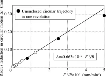
対象MCの場合,指令半径R(mm),指令送り速度F(mm/min)の円運動の半径減少量r(mm)はF2/Rに 比例する(丘他,1998).
R k F r 2/
(21) 上式を式(16)に代入して整理すると,MC駆動軸サーボ系時定数T(sec)と比例係数kとの関係は次式となる.
T 7200k (22) kの値を決めるために,対象 MCのXY平面において表1 に示す条件で円運動を行い,HEIDENHAIN社製の
KGM181型の交差格子測定装置を使用してその軌跡を測定する.得られた円運動軌跡の例を図5に示す.さらに,
KGM装置のISO 230-4:2005準拠の円運動精度評価機能を利用して各条件での円運動半径減少量を求める(ISO
230-4:2005).その結果を図6に示す.小さい半径と高い送り速度を指令した場合,駆動軸サーボ系の追従能力の
制限により,円運動一周の軌跡の両端が離れている例(図5(a)を参照)も見られるが,このような3条件の結 果を除外し,最小二乗法を用いて求めたkの値は0.663×10⁷である.したがって,対象MCの駆動軸サーボ系時
0 v
t vx,i Actual feed rate vx
vx,i1
Acceleration of the (i1)-th segment
Deceleration of the i-th segment
t t1 t2 X
Y
O F
Ci+1 Ci
Si Di
Ei=Si+1 Ri
Ri+1 Ei+1
The i-th circular arc segment
The (i+1)-th circular arc segment
Bi
Qiu, Transactions of the JSME (in Japanese), Vol.85, No.875 (2019)
Table 1 Parameters of measured circular motions.
R [mm] Feedrate F [mm/min] Rotation direction 5 500, 1000, 2000*, 5000*
Clockwise and counter-clockwise 10 500, 1000, 2000, 5000*
20 500, 1000, 2000, 5000 50
* Circular trajectory in one revolution does not enclosed.
Fig. 5 The measured circular motion trajectories by KGM device based on ISO 230-4:2005 standard. (a) shows an example where a trajectory in one revolution does not enclose, due to insufficient capacity of the servo axis to the specified motion conditions. (b) shows an example where both trajectories, one in CCW direction (red line) and another in CW direction (blue line), agree well with each other at the positions of 45 and 135 relative to the X axis. This means the X and Y axes have the same value of the time constant in servo system.
Fig. 6 The least-square estimation result for proportional coefficient k between r and F 2/R, where F, R and r are the specified values of feed rate and radius, and the radius reduction in the tested circular motion, respectively.
(a) R=5 mm, F=5000 mm/min, 20 m/div (b) R=10 mm, F=2000 mm/min, 10 m/div
4
3 5
Radius reduction in circular motionr(mm)
F 2/R106 (mm/min2)
r0.663107 F 2/R 0.30
2 0 1
0.10 0.20
●Unenclosed circular trajectory in one revolution
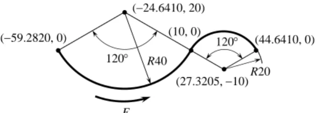
Fig. 7 Test cutter path for identifying t.
定数Tの値は0.0218 secとして定めることができた.なお,図5(b)に示すように,X軸に対して45と135の
位置において,同じ指令半径と送り速度の円運動の時計方向回り(CW)軌跡と反時計方向回り(CCW)軌跡が 重なっている.これは,X軸とY軸のサーボ系時定数の値が一致することを意味している(垣野他,1987).
3・2 円弧セグメントの加減速タイミングパラメータtの同定方法と結果
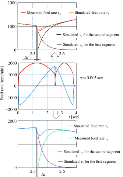
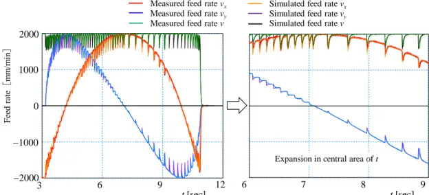
前後の円弧セグメントの加減速運動のタイミングを表すパラメータtの値を推定するために,図7に示す2円 弧工具経路の軌跡をKGM装置で測定する.KGM測定におけるサンプリングタイムを用いて,得られた軌跡の座 標データについて数値微分することにより,実際のMCのX軸とY軸の送り速度成分を求めることができる.F=
2000 mm/minを指令して得られたMC各軸の送り速度成分を図8に示す.前章に説明した円弧セグメントの加減
速運動関係および前節に定めたTの値に基づき,図8に示したKGM測定から得られた駆動軸の送り速度データ について,最小二乗法を利用して推定したtの値は0.005 secである.この結果を用いてつぎの4章に述べるシミ ュレーション方法で計算した送り速度成分の曲線も図8に記入している.図中にセグメント接続点の近辺に,計 算した送り速度曲線の急峻な変化に対して,KGM測定による送り速度成分曲線の変化が幾分緩やかに見えるが,
これはサンプリングタイムに係わる数値微分処理や駆動軸接触部の接触変形に及ぼす速度変化などの影響と考え られる.このような局部的違いを除けば,送り速度の計算結果と測定結果はよく一致していることがわかる.
F =2000 mm/minとF =5000 mm/minの場合でのKGM装置による運動軌跡の測定結果を図9に示す.同図には Tとtの同定結果に基づいて4章のシミュレーション方法から計算した2円弧工具経路の運動軌跡も記入してい る.実測運動軌跡曲線における Y 軸の方向入換時に発生するスティックモーションによる突起(垣野他,1986)
を除けば,計算結果は実測結果とよく一致していることがわかる.この結果から,パラメータの同定値は妥当で あると思われる.
4. 工具経路運動軌跡のシミュレーション方法 4・1 工具経路の記述とセグメントの加減速運動時間
図10に示すように,対象とするMCの工具経路はつながり点でドウェルを設けず,前後に接しているn個の 円弧セグメントで構成される.指令位置として工具経路の開始点をA0(X0, Y0),i番目(i1,2,,n)セグメン トの終了点をAi(Xi, Yi),半径をRi,中心点をCi(Xc, i, Yc, i),指令送り速度をFiとする.なお,i番目セグメント の中心角をiと記し,i番目セグメントの減速運動開始点をBi(xb, i, yb, i)で, i+1番目セグメントの加速運動開始 点をDi(xd, i, yd, i)で記述する.
第2章の説明と同様に各セグメントの加速運動時間tiは式(23)で決まる.
i i i
i R F
t /
(23)
また,簡潔のため,各セグメントの減速運動の時間TiはTとして統一的に取り扱う.
max( , , , ) /
log F1 F2 F T
T T
Ti e n
(24)
なお,各セグメントの関連パラメータは次のように定義される.
(59.2820, 0)
(24.6410, 20) (10, 0)
(27.3205, 10)
(44.6410, 0) R40
R20
F 120
120
Qiu, Transactions of the JSME (in Japanese), Vol.85, No.875 (2019)
Fig. 8 Estimation value of parameter t and feed rate components of servo axes in the identification experiment. The upper and lower graphs show an enlarged curve part of feed rate component respectively in the X axis and Y axis around the connection point of two segments.
Fig. 9 Comparison of simulated cutter paths with measured ones in the identification experiment for t. There is a good consistency between the both trajectory curves.
i i
i F /R
(25)
i ci i ci
i atan2 Y1Y, , X 1X ,
(26)
) tan( i
i T
(27)
810°
0 0
-250 Radial deviation [m]
Angle of measured point [deg]
250
180°
外側円弧(壁型)
回転数 = 送り速度 = 切り込み =
50000.00 rpm 5000.00 mm/min
5.00 mm
360° 540° 720°
切込み0mm
円弧の領域 駆動軸の切替位置
R20
切込み0.05mm の後 0 mm
t[sec]
2000 1000 0
1000
2000
0 1 2 3 4
Feed rate [mm/min]
t 2000
1000
0 2.5 2.6
810°
0 0
-250 Radial deviation [m]
Angle of measured point [deg]
250
180°
外側円弧(壁型)
回転数 = 送り速度 = 切り込み =
50000.00 rpm 5000.00 mm/min
5.00 mm
360° 540° 720°
切込み0mm
円弧の領域 駆動軸の切替位置
R20
切込み0.05mm の後 0 mm
810°
0 0
-250 Radial deviation [m]
Angle of measured point [deg]
250
180°
外側円弧(壁型)
回転数 = 送り速度 = 切り込み =
50000.00 rpm 5000.00 mm/min
5.00 mm
360° 540° 720°
切込み0mm
円弧の領域 駆動軸の切替位置
R20
切込み0.05mm の後 0 mm
t 2000
0 2.5 2.6
―
Measured feed rate vx―
Simulated feed rate vx―
Simulated vxfor the second segment―
Simulated vxfor the first segmentt=0.005 sec
―
Measured feed rate vy―
Simulated feed rate vy―
Simulated vyfor the second segment―
Simulated vyfor the first segment 凸型回転数 = 50000.00rpm 送り速度 = 5000.00mm/min 切り込み = 5.00mm
外側円弧 凸型
回転数 = 50000.00rpm 送り速度 = 5000.00mm/min 切り込み = 5.00mm
外側円弧
Measured path
Simulated path Commanded path
F=2000 mm/min F=5000 mm/min
4・2 工具経路運動軌跡のシミュレーションアルゴリズム
アルゴリズムには,区別のため,MCの運動開始からの累積時間をt,各セグメントの加速過程と減速過程を記 述する動作時間をと記す.
(a)i1とする.点A0から点B1までの駆動軸速度vx()とvy()を式(28)と(29),工具経路軌跡x()とy() を式(30)と(31)から計算する.
sin( ) sin( )
1 )
( 1 1 1 1 1
2 1 2
1
T
x e
T
v F (28)
cos( ) cos( )
1 )
( 1 1 1 1 1
2 1 2
1
T
y e
T
v F (29)
1 1 1 1 1
01 1
2 1 1 2
1 1 cos( ) cos( )
) 1 )(
sin(
1 )
( T e X
T
x F T
(30)
1 1 1 1 1
01 1
2 1 1 2
1 1 sin( ) sin( )
) 1 )(
cos(
1 )
( T e Y
T
y F T
(31)
ただし,動作時間は次式による.
0 tt1 (32)
一方,点B1から点D1までの駆動軸速度を式(33)と(34),工具経路軌跡を式(35)と(36)から計算する.
T T
t
x e t e
T v F
sin( ) sin( )
1 )
( 1 1 1 1 1 1
2 1 2
1
1
(33) Fig. 10 The cutter path composed of circular arc segments.
Y
F1 A0 A1
A2
A3
C1
X C3
C2
An Cn
R1 R2 R3
Rn
F2 O
F3 Fn1
Fn
Bn
B1 B2
D1
D2 B3 D3
Rn1
Cn1
An1 n
n1
3
2
1
Qiu, Transactions of the JSME (in Japanese), Vol.85, No.875 (2019)
T T
t
y e t e
T v F
cos( ) cos( )
1 )
( 1 1 1 1 1 1
2 1 2
1
1
(34)
1 1
1 1 1 1
2 1 1 2
1 sin( ) sin( ) (1 )
1 )
(
1
b T T
t
x e t
e T
T
x F
(35)
1 1
1 1 1 1
2 1 1 2
1 cos( ) cos( ) (1 )
1 )
(
1
b T T
t
y e t
e T
T
y F
(36)
ただし,動作時間は次式による.
t t t
1
0 (37)
(b)ii1と置き換える.点Di1から点Biまでの駆動軸速度と工具経路軌跡をそれぞれ式(38)と(39)お よび式(40)と(41)から求める.
1
2 2 2 2
1
) sin(
) sin(
1
) sin(
) sin(
1 )
(
i
J j
T t t t j j j j T
t j j j
j
i i i T
i i i
i x
j i j
e t
e T
F
e T
v F
(38)
1
2 2 2 2
1
) cos(
) cos(
1
) cos(
) cos(
1 )
(
i
J j
T t t t j j j j T
t j j j
j
i i i T
i i i
i y
j i j
e t
e T
F
e T
v F
(39)
1
2 2
1 2 ,
2
) 1 ( )
sin(
) sin(
1
) cos(
) 1 cos(
) 1 )(
sin(
1 )
(
i 1
J j
T T
t t t j j j j T
t j j j
j
i d i i i
i i i T
i i i
i
e e
t e
T T F
x e
T T
x F
j i
j
(40)
1
2 2
1 2 ,
2
) 1 ( )
cos(
) cos(
1
) sin(
) 1 sin(
) 1 )(
cos(
1 )
(
i 1
J j
T T
t t t j j j j T
t j j j
j
i d i i i
i i i T
i i i
i
e e
t e
T T F
y e
T T
y F
j i
j
(41)
ただし,動作時間は次式による.
i
i t t
t
t
1
0 (42)
式中のti1は次のように決める.
2
1
1
1 ( )
i
j
i j
i t t t
t (43)
また,式(38)~式(41)におけるJは次式を満たす最小のjとする.
) 1 , , 2 , 1
1 (
t T t j i
ti j (44)
(c)点Biから点Diまでの駆動軸速度と工具経路軌跡をそれぞれ式(45)と(46)および式(47)と(48)か ら計算する.
i
J j
T t t j j j j T
t j j j
j x
j i j
e t
e T
v F
sin( ) sin( )
1 )
(
2
2 (45)
i
J j
T t t j j j j T
t j j j
j y
j i j
e t
e T
v F
cos( ) cos( )
1 )
(
2 2
(46)
i
J j
i b T T
t t j j j j T
t j j j
j e t e e x
T T x F
j i j
2 ,
2 sin( ) sin( ) (1 )
1 )
(
(47)
i
J j
i b T T
t t j j j j T
t j j j
j e t e e y
T T y F
j i j
2 ,
2 cos( ) cos( ) (1 )
1 )
(
(48)
ただし,動作時間はセグメントの番号に応じて次の式による.
n i t t
t i
, for
0 (49) n
i T
t
t n
, for
0 (50)
(d)inなら(b)へ戻る.inならば計算を終了する.
上述のように,各セグメントの加速運動の動作時間ti,減速運動開始から次のセグメントの加速運動開始まで の時間t,および各セグメントの減速運動の動作時間Tが前もって簡単に決められるので,提案アルゴリズムに 基づく計算プログラムの作成は簡単にできる.
5. 工具経路運動軌跡推定結果の実験検証
提案したシミュレーション方法の妥当性を確認するために,KGM測定装置を使用して測定するMCの工具経 路運動軌跡および三次元測定機(以下,CMM と略す)を使用して測定する仕上げ加工ワークの輪郭を同じ運動 条件でシミュレーションする工具経路の軌跡と比較する.
輪郭切削実験には,ナカニシ製のドライバー付き高速スピンドルをMCの主軸に装着し,そのチャックにエン ドミルを取り付ける.切削中にMCの主軸を回転させずに高速スピンドルによって工具を回す.一方,ワーク材 をMCのテーブルに取り付け,NCプログラムでテーブルを駆動する.使用するエンドミルの直径は3 mmで,
切削中に工具径のオフセット補正をしない.
仕上げ加工したワーク輪郭の測定においてミツトヨ製のBHN506型CMMと先端直径3 mmのタッチトリガー プローブを使用する.測定中にプローブ径の補正処理をしないので,得られた輪郭データはそのまま加工中の工 具経路に対応している.
Qiu, Transactions of the JSME (in Japanese), Vol.85, No.875 (2019)
Table 2 Machining conditions for contouring.
Cutting conditions
Spindle speed N [rpm] / Feedrate F [mm/min] 50,000 / 5,000, 20,000 / 2,000, 10,000 / 1,000
Radial depth of cut [mm] 0 after 0.02
Axial depth of cut [mm] 5
Cutting direction / Fluid Down cutting / Wet
End mill
Diameter [mm] 3
Flute number 2
Helix angle [] 30
Material CO-HSS + TiN coating
Work piece Material Aluminium A5052
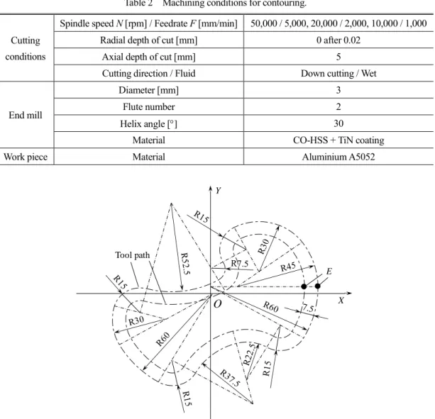
Fig. 11 Cutter path 1 used in verification experiments, which is composed of 13 circular arc segments respectively for the outer side or the inner side and a dwell action of 1 second is specified at the start and end point, point E, of each side.
5・1 工具経路 1 の検証実験結果
検証実験に二つの工具経路を使用する.工具経路1を図11に示す.それは法線距離7.5 mmの二つのオフセッ ト曲線であり,それぞれ接続点で接する13個の円弧で構成されている.点Eは工具経路の開始点と終了点であ り,運動開始時と終了時にこの点で1秒間ドウェルを設けている.CWとCCWの両送り方向に表2に示す運動 条件を指令して外側と内側の工具経路を別々に動かし,その運動軌跡を測定する.また,同じ運動条件のもとで 同表に示す切削パラメータを用いてワーク輪郭を仕上げる.
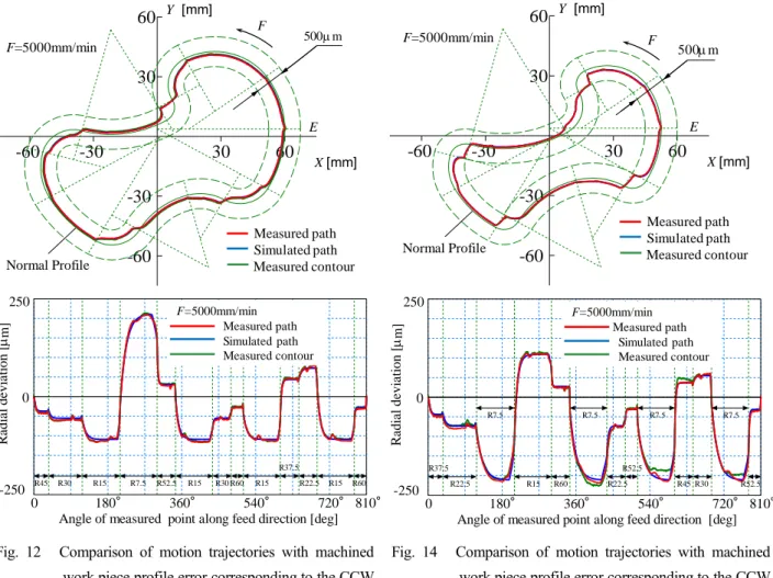
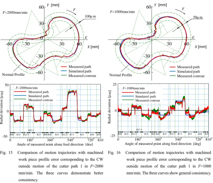
図12にCCW方向の指令送り速度F=5000 mm/minの外側工具経路の実測結果とシミュレーション結果との比 較を示す.上の図にワークの輪郭にそって誤差を示している.下の図には縦軸が測定点の誤差,横軸が工具経路 の開始点から測定点までの補間円弧沿いの回転角累積値を示す.円弧接続点のまわりに段差状の運動誤差が見ら れる.円弧の指令半径値が小さければその両端に半径減少による段差が大きくなり,凹凸が逆になる円弧の接続 点のまわりに,両側円弧の半径減少量の和に等しい大きな段差が発生する.なお,実測軌跡曲線において,MC駆 動軸の進行方向が入れ替わるたびにスティックモーションによる突起が見られる.特にドウェル動作を設けた工 具経路の終始点Eでの突起が大きい.これは円運動の半径減少量とスティックモーションによる突起が重なった からである.図からわかるように,運動軌跡の実測結果とシミュレーション結果および同図に記入している加工 ワークの輪郭誤差曲線の三者がよく一致している.
凸型
回転数 = 10000.00rpm 送り速度 = 5000.00mm/min 切り込み = 0.02mm
内側円弧
実測値
誤差スケール値 測定経路
シミュレーション値 の後 0 mm
円弧領域線
E Tool path
O
Y
X
Qiu, Transactions of the JSME (in Japanese), Vol.85, No.875 (2019)
Fig. 12 Comparison of motion trajectories with machined work piece profile error corresponding to the CCW outside motion of the cutter path 1 in F=5000 mm/min. The three curves demonstrate good consistency.
Fig. 14 Comparison of motion trajectories with machined work piece profile error corresponding to the CCW inside motion of the cutter path 1 in F=5000 mm/min. The three curves demonstrate good consistency.
Fig. 13 Measured feed rate and its components along each servo axis, which are obtained by a numerical differentiation operation to the coordinate data of the measured cutter path trajectory shown in Fig. 12. These curves demonstrate good consistency relative to the simulated ones.
図12の実測工具経路の座標データについて数値微分して求めた MCの各駆動軸の送り速度成分vx,vyおよび 送り速度の値v vx2v2y を図13に示す.シミュレーションによる送り速度も同図に記入している.セグメント 間の接続点に対応する曲線突起点の位置において,数値微分の影響によりシミュレーション結果とKGM測定結 果に突起の大きさが違う箇所も見られるが,全般的に両者はよく一致している.
810°
0 0
-250 Radial deviation [m]
Angle of measured point along feed direction [deg]
250
180° 360° 540° 720°
R45 R30 R15 R7.5 R52.5 R15 R30R60 R15 R37.5
R22.5
R20 R15 R60
F=5000mm/min Measured path Simulated path Measured contour
-60 -30 30 60
-60 -30 30 60
X[mm]
Y [mm]
回転数 = 10000.00rpm 送り速度 = 5000.00mm/min 切り込み = 0.02mm
実測値 誤差スケール値 測定経路
シミュレーション値
500m の後 0 mm
円弧領域線
Normal Profile F=5000mm/min
F
Measured path Simulated path Measured contour
E
810°
0 0
-250 Radial deviation [m]
Angle of measured point along feed direction [deg]
250
180° 360° 540° 720°
R37.5 R52.5
R22.5 R7.5
R15 R60 R7.5
R22.5 R7.5
R45 R30
R20 R52.5
R7.5
F=5000mm/min Measured path
Simulated path Measured contour
-60 -30 30 60
-60 -30 30 60
X[mm]
Y [mm]
回転数 = 10000.00rpm 送り速度 = 5000.00mm/min 切り込み = 0.02mm
実測値 誤差スケール値 測定経路
シミュレーション値
500m の後 0 mm
円弧領域線
Normal Profile
F=5000mm/min F
Measured path Simulated path Measured contour
E
Feed rate [mm/min]
5000 2500
2500
5000
0 1.05 2.1 3.15 4.2
t[sec]
0
外側円弧(壁型)
回転数 = 送り速度 = 切り込み =
50000.00 rpm 5000.00 mm/min 5.00 mm
切込み0mm
円弧の領域 駆動軸の切替位置
R20
切込み0.05mm の後 0 mm
Measured feed rate vx Measured feed rate vy Measured feed rate v Simulated feed rate vx Simulated feed rate vy Simulated feed rate v