PAPER
A Heuristic Algorithm for Solving the Aircraft Landing Scheduling Problem with a Landing Sequence Division
Wen SHI†a),Member, Shan JIANG††, Xuan LIANG†,andNa ZHOU†,Nonmembers
SUMMARY Aircraft landing scheduling (ALS) is one of the most im- portant challenges in air traffic management. The target of ALS is to decide a landing scheduling sequence and calculate a landing time for each aircraft in terminal areas. These landing times are within time windows, and safety separation distances between aircraft must be kept. ALS is a complex prob- lem, especially with a large number of aircraft. In this study, we propose a novel heuristic called CGIC to solve ALS problems. The CGIC consists of four components: a chunking rule based on costs, a landing subsequence generation rule, a chunk improvement heuristic, and a connection rule. In this algorithm, we reduce the complexity of the ALS problem by breaking it down into two or more subproblems with less aircraft. First, a feasi- ble landing sequence is generated and divided into several subsequences as chunks by a chunking rule based on aircraft cost. Second, each chunk is regenerated by a constructive heuristic, and a perturbative heuristic is applied to improve the chunks. Finally, all chunks constitute a feasible landing sequence through a connection rule, and the landing time of each aircraft is calculated on the basis of this sequence. Simulations demonstrate that (a) the chunking rule based on cost outperforms other chunking rules based on time or weight for ALS in static instances, which have a large number of aircraft; (b) the proposed CGIC can solve the ALS problem up to 500 aircraft optimally; (c) in dynamic instances, CGIC can obtain high-quality solutions, and the computation time of CGIC is low enough to enable real-time execution.
key words: air traffic management, aircraft landing scheduling, heuristic
1. Introduction
Aircraft fly into a terminal area from different routes to land on the runways of the airport. A scheduled landing time is allocated to each aircraft by a controller because aircraft may be unable to land at the planned arrival time. The scheduled landing time is in the time window, which is between the earliest and the latest landing time of the aircraft. Scheduled landing time separations between aircraft must be no less than safety standards because of wake turbulence and other factors. Therefore, the scheduled landing time of an aircraft may not be exactly equal to the target landing time. In air- craft landing scheduling (ALS) problem, the objective is to minimize the total deviation of the scheduled landing time from the target landing time for each aircraft, whereas the scheduled landing time is in time window, and the separation constraints are satisfied. Obviously, the more the aircraft in- terfere with one another, the more complex the ALS problem will be.
Manuscript received November 20, 2018.
Manuscript revised March 13, 2019.
†The authors are with the Tianjin University of Commerce, China.
††The author is with the Tianjin Medical University, China.
a) E-mail: [email protected] DOI: 10.1587/transfun.E102.A.966
Numerous attempts have been made to solve an ALS problem. These approaches can be classified into two cat- egories: exact algorithm and heuristic algorithm. Beasley et al.[1]presented a mixed-integer zero-one formulation of ALS problems and performed a linear programming-based tree search to solve them. Faye et al.[2]proposed a method based on the approximation of a separation time matrix and on time discretization to solve ALS problems.
Many heuristics are proposed to solve ALS problems.
Sabar et al.[3]proposed an iterated local search algorithm, which is a single-solution-based search methodology, to min- imize the total penalty of landing deviations from the tar- get landing time. Beasley et al.[4]developed a population heuristic to schedule aircraft landings at London Heathrow.
In 2006, two heuristic techniques, namely, scatter search and bionomic algorithm, were presented for ALS problems[5].
The two population heuristic algorithms were applied to test instances involving up to 500 aircraft.
Some studies have introduced a heuristic by using a local search to obtain a scheduled landing sequence, and an exact algorithm to calculate the landing time of each aircraft based on this landing sequence. Ernst et al.[6]de- veloped a heuristic approach and a simplex algorithm to calculate the upper and lower bounds of a branch-and-bound scheme to evaluate solutions. Hu et al.[7] designed a ge- netic algorithm based on a binary representation of arriving sequences. Yu et al.[8]proposed a cellular automata opti- mization(CAO), which consists of three components: a cel- lular automata model to generate a landing sequence, a local search to improve the landing sequence, and a deterministic operator to calculate the optimal landing times based on the landing sequence. Salehipour et al.[9] designed a hybrid meta-heuristic applying a simulated annealing framework.
The framework includes a problem-dependent construction heuristic and a variable neighborhood descent meta-heuristic with three neighborhood structures as an improvement algo- rithm. In 2014, we proposed a dynamic hyper-heuristic algorithm for the ALS problem [10]. A scatter search is adopted as a high level heuristic, which builds a chain of priority rules as low level heuristics to generate a landing sequence.
The longer the landing sequence generated by a heuris- tic algorithm is, the larger the computation time of the exact algorithm for calculating the landing time of each aircraft will be. Therefore, the set of aircraft can be divided into several subsets, called chunks. The landing time of each aircraft in every chunk is calculated, and the computation Copyright © 2019 The Institute of Electronics, Information and Communication Engineers
time is short enough even in dynamic ALS instances. Furini et al.[11],[12] proposed three chunking rules to generate chunks with a length constraint and found that different rules iteratively applied to various sequences can obtain better re- sults than those determined without chunking or those with a single chunking rule.
In this study, we proposed a novel algorithmCGICto solve ALS problems. Our approach consists of four compo- nents: a chunking rule based on costs (C Rcost), a landing subsequence generation rule (GR), a chunk improvement heuristic (I H), and a connection rule(C N R). First, a land- ing sequence generated by a non-optimization method First- Come-First-Served (FCF S) is divided into several chunks through the chunking rule. Chunking rules proposed in[12]
are based on time or weight and with constraints of length of chunks. C Rcost is based on cost of each aircraft and without any constraints of length. Therefore,C Rcost aims to place most aircraft that interfere with one another in the same chunk. Second, all aircraft in one chunk are resched- uled byGR.GRis based on cost priority. The aircraft with a larger cost is inserted into a new landing subsequence in the chunk with a higher priority. Third, the generated landing subsequence is improved usingI H. InI H, the aircraft with the highest cost in the subsequence is selected, and several aircraft that land continuously before or after this aircraft with the highest cost are resequenced randomly to decrease the total cost of the subsequence. Finally, all of the subse- quences in every chunk are combined into a complete final landing sequence throughC N Rand the landing time of each aircraft is calculated by using an exact algorithm based on the final landing sequence.
The remaining parts of this paper are organized as fol- lows: Section 2 describes the problem statement. Section 3 provides the details of the proposed algorithmCGIC. Sec- tion 4 reports the simulation results to evaluate the efficacy of theCGIC. Section 5 concludes this paper and presents recommendations for some future work.
2. Aircraft Scheduling Landing: Problem Definition The ALS problem is divided into two types: static and dy- namic. We formulate the static and dynamic ASL problems as mixed integer linear problems. Thus, parameters and variables are defined as follows:
Parameters:
• Fall: the set of all aircraft.
• Ff : the set of aircraft that are scheduled to land and could not be rescheduled.
• Fs : the set of aircraft that are scheduled to land and could be rescheduled during an update.
• Fa : the set of aircraft scheduled to land and Fa = Ff ∪Fs.
• Tit: the target landing time of aircrafti.
• Tia: the appearance time of aircrafti.
• Tie: the earliest landing time of aircrafti.
• Til: the latest landing time of aircrafti.
• Si j: the separation time between aircraftiand jwhen aircraftilands before j.
• c−i : penalty cost per unit of time for landing before target time of aircrafti.
• c+i : penalty cost per unit of time for landing after target time of aircrafti.
• Tf : the freeze time in which a scheduled landing time allocated for any aircraft withinTf of the current time could not be rescheduled.
Variables:
• xi : the scheduled landing time of aircrafti.
• δi j : a Boolean variable; if aircraftilands before j, it takes 1.
• tcur : the current time.
2.1 Static Model
In a static model, all aircraft appear and can be scheduled.
Therefore,Fs =Fa =Fall. No aircraft is frozen to allocate a scheduled landing time, that is, Ff =∅. For each aircraft inFs, the scheduled landing timeximust be within the time window:
Tie≤xi ≤Til (i∈Fs). (1) The landing time of any two aircraft in Fs must meet the safety standards:
(xj−xi) ≥Si j−M∗δji (i∈Fs,j ∈Fs,i,j). (2) where M is a sufficiently large number used to ensure that Eq. (2) is redundant in the case when aircraft jlands before i(δji=1). The objective function minimizes the total cost of landing deviation from the target landing time of each aircraft inFs.
Min z= X
i∈Fs
zi zi =
( ci−(Tit−xi) if xi ≤Tit ci+(xi−Tit) if xi >Tit.
(3)
2.2 Dynamic Model
In a dynamic ALS problem, all aircraftFallconsists of air- craft inFaand aircraft that have no appearance. Aircraft that have no appearance do not affect scheduling aircraft in Fa. Fa can be divided into two parts: Ff andFs. InFf, aircraft are too close to land at the current time and landing time cannot be further changed. Thus, the dynamic ALS model contains not only inequality (1)(2) but also other constraints, such as
Ff ={i|xi−tcur <Tf}. (4) In every iteration, the landing time of aircraft inFsis calcu- lated. When an aircraft is frozen, it no longer appears inFs. Thus,
Fs=Fa−Ff. (5) All aircraft in Fs must land after the aircraft in Ff. The scheduled landing time xi of aircrafti inFs is larger than any landing timexj of aircraft j, which is inFf. Therefore, the lower bound of the time window is as follows:
xi ≥M ax(Tie,xj) (i∈Fs,j ∈Ff). (6) The separation time between an aircraft inFsand an aircraft inFf must be satisfied:
(xi−xk)≥Ski (i∈Fs,k∈Ff). (7) The objective function in the dynamic model is the same as in the static model.
3. C GI CAlgorithm
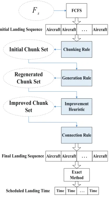
TheCGIC algorithm proposed in this study contains four main components:C Rcost,GR,I H, andC N R. First,FCF S generates an initial landing sequence from Fs. Second, the initial landing sequence is divided into several chunks by C Rcost. Third, aircraft are rescheduled in each chunk throughGR. Furthermore, the rescheduled chunks are im- proved using the perturbative heuristicI H. Subsequently, C N Rconnects all chunks and constructs the final landing sequence. Finally, an exact method calculates the landing time of all aircraft based on the final landing sequence. The flowchart of theCGICalgorithm is shown in Fig. 1. Some variables and parameters in the algorithm are defined as fol- lows:
• seqini: the initial landing sequence.
• seqf in: the final landing sequence.
• seqt: the landing subsequence of chunkt.
• seq(p): thepth aircraft inseq.
• xseq(p): the landing time of thepth aircraft inseq.
• cost(seq(p)): the cost of thepth aircraft inseq.
• cost(seq): the sum of the cost of each aircraft inseq.
• |seq|: the length of the landing sequenceseq.
• F(p): thepth aircraft inF.
• |F|: the number of aircraft in aircraft setF.
• Cini: the initial chunk set.
• Cimp: the improved chunk set.
• |C|: the number of chunks in chunk setC.
3.1 The Chunking Rule
The proposedC Rcost procedure aims to collect some ad- jacent aircraft in seqini into a chunk and does not affect the landing time of the aircraft in other chunks as much as possible. For example, some adjacent aircraft are se- lected. The costs of the first and last aircraft are 0 and the total cost of these aircraft without constraints from the other aircraft in seqini is equal to the sum of the costs of the same aircraft in the initial landing sequence. Then these aircraft have less impact on the other aircraft because the
Fig. 1 Flow ofCGICalgorithm.
total cost is unchanged after these aircraft are selected out of seqini. Therefore, in contrast to other chunking rules, such as C Rf ixed,C Rtime, andC Rweight proposed in [11],[12], C Rcostgenerates chunks based on the cost of aircraft with- out any length constraints. C Rcostmeasures the cost of each aircraft inseqini and selects a subsequenceseqpq. In this subsequence, the costs of the first aircraft seq(p) and the last aircraft seq(q) are 0. If cost(seqpq) is equal to the sum of the costs of the same aircraft inseqini, the aircraft in this sequence have less impact to the other aircraft inseqini. Furthermore, the subsequence is taken as a new chunk into the Cini. If the total cost of the subsequence is not equal to the sum of the original cost of the same aircraft, more aircraft are added to this subsequence until two conditions are satisfied: the costs of the first and the last aircraft in the subsequence are 0, and the total cost of this subsequence is equal to the sum of the costs of the same aircraft in seqini. Two adjacent chunks share the same aircraft. This aircraft
Algorithm 1:The Pseudo Code ofC Rcost
1 Setp=0;q=p+1;p,qare the index of aircraft inseqi ni;
2 whilep<q≤ |Fs|do
3 if (cost(seqi ni(p))=0| |p=0)&cost(seqi ni(q))=0 then
4 Generate a subsequenceseqp q, which contains aircraft from thepth to theqth inseqi ni;
5 Calculate a landing time of each aircraft inseqp q without constraints from the other aircraft inseqi ni;
6 if cost(seqp q)=Pq
k=pcost(seqi ni(k))then
7 Construct the subsequenceseqp qas a new chunk and place it inCi ni;
8 p=q;
9 q=q+1 ;
10 Continue ;
11 end
12 else
13 if∃r,p≤r ≤q & xs e qp q(r)<xs e qi ni(r) then
14 Get the subsequenceseqs pwhich is before seqp q;
15 Connect the two subsequences as a new subsequence and setp=s;
16 Continue ;
17 end
18 end
19 end
20 q=q+1 ;
21 end
can be seen as a key node aircraft, and its cost is 0.
3.2 The Generation Rule
After all chunks are constructed from seqini, each chunk inCini is regenerated, that is to say, aircraft in one chunk are rescheduled byGR. InGR, the aircraft with the largest cost in the chunk is selected and tried to be inserted into a new sequence. If this aircraft conflicts with other aircraft in the new sequence based on its target landing time, the aircraft with the largest cost tries to replace these conflicted aircraft in the new sequence. If the cost of the new sequence decreases after the replacement is completed, the conflicted aircraft is removed from the new sequence and placed in the unscheduled aircraft set. When all of the conflicted aircraft are replaced, the aircraft with the largest cost can be inserted into the new sequence with its target landing time. Otherwise, the aircraft with the largest cost is inserted into the new sequence at a scheduled landing time, and the landing time of the other aircraft is unchanged.
3.3 The Improvement Heuristic
InI H, every chunk is improved to decrease its cost by dis- ordering a subsequence before or after the aircraft with the largest cost. If the aircraft lands after its target landing time, the subsequence to be disordered contains some aircraft land- ing before this aircraft and the aircraft with the largest cost.
Conversely, the subsequence contains the aircraft with the
Algorithm 2:The Pseudo Code ofGR
1 for t=0 to|Ci ni|do
2 for p=0 to seqt
do
3 Calculatexs e qt(p)andcost(seqt(p));
4 end
5 Place all of the aircraft inseqtin a unscheduled setFu n;
6 Construct an empty landing sequenceseqnewas a new chunk;
7 whileFu n,∅do
8 Get aircraftjinFu nwhile the cost ofjis maximum in seqt;
9 Find all of the aircraft inseqnewwhich have conflict withjand place them in a setFc;
10 forq=0 to|Fc|do
11 Copy theseqnewas a new sequenceseq0;
12 Replace the aircraftFc(q)with aircraftjinseq0;
13 ifcost(seq0)≤cost(seqnew)then
14 PutFc(q)intoFu n;
15 RemoveFc(q)fromFcandseqnew;
16 end
17 end
18 ifFc =∅then
19 Insert aircraftjintoseqnewwith the landing timeTjt;
20 end
21 else
22 Calculate a landing time with minimum cost for aircraftjbased on the landing time of the other aircraft inseqnew;
23 Insert aircraftjintoseqnewwith the calculated landing time;
24 end
25 end
26 ifcost(seqnew)≤cost(seqt)then
27 seqt=seqnew;
28 end
29 end
largest cost and those landing after it when the aircraft with the largest cost lands earlier than its target time. The length of the subsequence is limited. After the subsequence is con- structed, three aircraft are selected and swapped randomly.
If the cost of the disordered chunk is not smaller than the original one, a new subsequence with a shorter length is constructed until the length of the subsequence is 3.
3.4 The Connection Rule
C N Rconstructsseqf inby connecting all of the chunks. In two adjacent chunks, if the last aircraft in the front chunk and the first aircraft in the later chunk are the same key node aircraft, one of the key node aircraft is removed, and the two chunks are connected to a new chunk. If the two aircraft are not the same, C N R connects two chunks and tries to generate two temporary sequences. One is constructed by removing the key node aircraft in the front chunk, and the other is constructed by removing the key node aircraft in the back chunk. The temporary sequence with an enhanced cost is chosen as a new sequence.
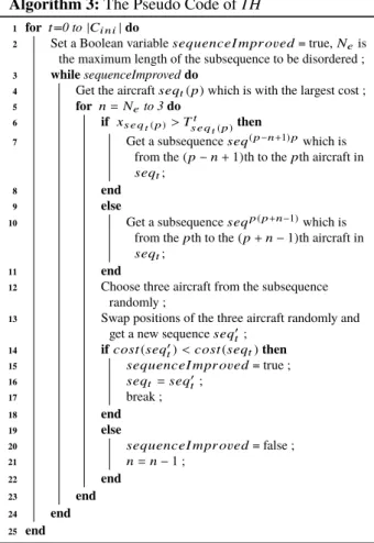
Algorithm 3:The Pseudo Code ofI H
1 for t=0 to|Ci ni|do
2 Set a Boolean variablesequenceI mpr oved= true,Neis the maximum length of the subsequence to be disordered ;
3 whilesequenceImproveddo
4 Get the aircraftseqt(p)which is with the largest cost ;
5 for n=Neto 3do
6 if xs e qt(p)>Ts e qt
t(p)then
7 Get a subsequenceseq(p−n+1)pwhich is from the(p−n+1)th to thepth aircraft in seqt;
8 end
9 else
10 Get a subsequenceseqp(p+n−1)which is from thepth to the(p+n−1)th aircraft in seqt;
11 end
12 Choose three aircraft from the subsequence randomly ;
13 Swap positions of the three aircraft randomly and get a new sequenceseqt0;
14 ifcost(seq0t)<cost(seqt)then
15 sequenceI mpr oved= true ;
16 seqt =seq0t;
17 break ;
18 end
19 else
20 sequenceI mpr oved= false ;
21 n=n−1 ;
22 end
23 end
24 end
25 end
4. Computational Experiments
4.1 Simulation Environment
Our computational tests use two types of instances. The first includes static instances. In these instances, all aircraft information is known whether or not it enters the termi- nal area. Therefore, all aircraft are scheduled only once, and the result is not changeable by time. The second com- prises dynamic instances. The aircraft that appear in the terminal area and not frozen are scheduled. The algorithm updates the landing sequence and the landing time for each aircraft in every time unit. All of the data of 13 instances with different numbers of aircraft of OR-Library[13]can be obtained at http://people.brunel.ac.uk/~mastjjb/
jeb/info.html. The ILOG’s CPLEX is used as the exact method to calculate the landing time for each aircraft based on the landing sequence. The computer runs on Intel Core i7-6500U 2.50 GHz, 2.50 GHz, 8 GB RAM, and Microsoft Windows 7.
4.2 Static Instances
First, we evaluate the performance of our proposed algo- rithmCGIC. The best results over the 30 replications of
Algorithm 4:The Pseudo Code ofC N R
1 Construct an empty landing sequenceseqf i n;
2 Addseq0intoseqf i n;
3 fort=1to
Ci m p
do
4 ifseqt−1( seqt−1
−1)=seqt(0)then
5 Removeseqt(0)fromseqt;
6 Addseqtto the end ofseqf i n;
7 end
8 else
9 Construct a new sequenceseqf r o nt=seqf i n;
10 Remove the key node aircraft from theseqf r o nt;
11 Addseqtto the end ofseqf r o nt;
12 Construct a new sequenceseqb eh i n d=seqf i n;
13 Remove the key node from theseqt;
14 Addseqtto the end ofseqb eh i n d;
15 ifcost(seqf r o nt)≤cost(seqb eh i n d)then
16 seqf i n=seqf r o nt;
17 end
18 else
19 seqf i n=seqb eh i n d;
20 end
21 end
22 end
Table 1 Best results of different approaches in static instances 1-9.
N FC F S C AO H H SS I LS CGIC
1 10 700 0.00 0.00 0.00 0.00
2 15 1500 1.33 1.33 1.33 1.33
3 20 1730 52.60 52.60 52.60 52.60
4 20 2520 0.00 0.00 0.00 0.00
5 20 5420 42.80 42.80 42.80 42.80
6 30 24442 0.00 0.00 0.00 0.00
7 44 1550 0.00 0.00 0.00 0.00
8 50 2480 21.17 21.37 21.37 21.37
9 100 7310 23.24 23.24 23.24 23.24
CGIC are compared with several previous approaches, in- cludingFCF S,C AO[8],H H SS[10], andI LS[3], in static instances. Nis the number of aircraft in different instances.
The results ofC AO,H H SS,I LS, andCGIC, in terms of the percentage gap from the best results ofFCF Sare calcu- lated as follows: (BRFC F S−BR)/BRFC F S∗100%, where BRFC F Sis the best result ofFCF S, andBRis the best result of the other algorithms.
In Table 1,CGICcan obtain the same optimal results as other algorithms in instances 1-9. In Fig. 2, the results of CGIC are not the best in all of the algorithms in instances 10 and 11. However,CGICobviously outperforms the other algorithms in instances 12 and 13, which have a large number of aircraft.
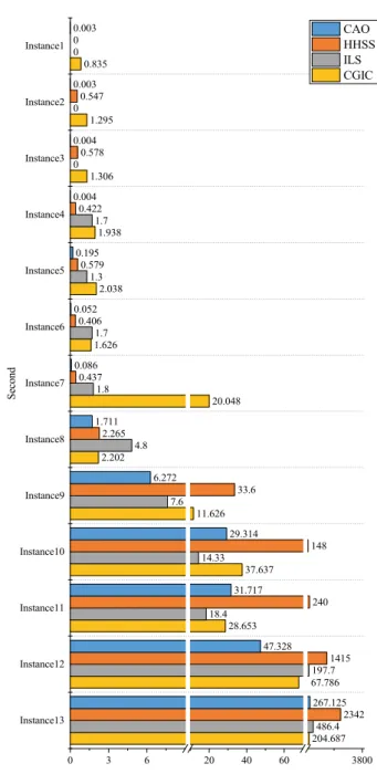
Figure 3 shows the average computation time over 30 replications ofCGICwith other algorithms. When the num- ber of aircraft is small, the computation time of CGIC is about 1 second except in instance 7. In instances 9-13, the computation time increases as N enlarges. When the num- ber of aircraft is 500 in instance 13, the average computation time ofCGICis shorter than that of other algorithms.
Figure 4 shows the average computation time of the four
Fig. 2 Best results of different approaches in static instances 10-13.
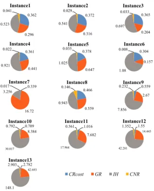
components (C Rcost,GR,I H, andC N R) ofCGIC.C Rcost andC N Rare fast algorithms because their computation time is short, especially in instances with a large number of air- craft. As a perturbation heuristic, the computation time of I Hoccupies most of the total time in most instances except instance 7.
Figure 5 shows the comparison of three different chunk- ing rules, namely,C Rtime,C Rweight, andC Rcost. First, each chunking rule generates an initial chunk set. Second,seqf in is constructed byC N R. The landing time is calculated by CPLEX based onseqf in. Finally, the percentage gaps from the best results ofFCF Sare shown in instances 9-13, which have a large number of aircraft. In most instances,C Rcost outperforms the two other chunking rules. In instance 11, the result ofC Rcostis equal to that ofC Rtime.
Ne is the maximum length of the subsequence to be disordered randomly, and it is considered an important pa- rameter inI H. Figure 6 shows the average results generated byCGICwith different Ne. These results are calculated in terms of the percentage gap from the best results ofFCF S:
(BRFC F S−AR)/BRFC F S∗100%, whereARis the average result generated by CGIC with different Ne. The experi- mental results in Fig. 6 demonstrate that better results can be generated when Ne is 6. If Ne is too small, I H, as a perturbative heuristic, cannot easily escape local optima. A largeNeindicates a long subsequence, which contains more aircraft. Disordering only three aircraft has less impact on the cost of the subsequence.
4.3 Dynamic Instances
We compare CGIC with different ∆t in 13 dynamic in- stances. ∆t is the unit of time. The freeze timeTf is set at 300 second. Table 2 shows the average results in instances 1-7 over the 30 replications ofCGIC. The results show the percentage gap from best results of FCF S. Different∆t, including 360, 480, and 600 seconds, are chosen. Table 2 shows that the results with different∆tof instances 1-7 and the results in static instances 1-7 are the same because the
Fig. 3 Computation time of different approaches (second).
number of aircraft in instances 1-7 is small, andCGICwith different∆tcan calculate the results as in the static instances.
Fig. 7 shows that the result with∆t600 seconds is the same as that of static instance 8, and the results with∆t 360 and 480 seconds are worse. The number of aircraft in instance 8 is 50, and the total time from the appearance time of the first aircraft to the latest landing time of the last aircraft is 828 seconds, which is close to the∆twith 600 seconds. There- fore,CGICwith a large∆tcan generate much better results in instance 8. However, the number of aircraft is larger with longer total time from instances 9 to 13. For example, the total time in instance 9 is 14,122 seconds. ∆twith 360, 480, and 600 seconds are much shorter than the total time. In instances 9 to 12, the results of∆twith 480 are optimal. The results of∆t with 360 seconds are not the best, indicating
Fig. 4 Computation time ofC Rc o s t,GR,I H, andC N Rin the total computation time ofCGIC(second).
Fig. 5 Best results of different chunking rules.
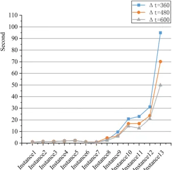
that the number of aircraft to be scheduled in Fs is small if∆t is small. Moreover, the landing time is calculated on the basis of less constraints from the other aircraft inFa in early ∆t. In later ∆t, aircraft have larger deviations from their target landing time. In instance 13, the result of∆twith 600 is optimal when the number of aircraft is 500, and the total time from the appearance time of the first aircraft to the latest landing time of the last aircraft is 56,382 seconds.
Figure 8 shows the average computation time over the 30 replications ofCGICwith different∆t. In dynamic in- stances, with a small number of aircraft, the average cal- culating time is close to static instances except instance 7.
However, the results in dynamic and static instance 7 are the same. When the number of aircraft is large, the average
Fig. 6 Effects ofNe.
Table 2 Average results in dynamic instances 1-7 with different∆t.
N 360 480 600
1 10 0.00 0.00 0.00
2 15 1.33 1.33 1.33
3 20 52.60 52.60 52.60
4 20 0.00 0.00 0.00
5 20 42.80 42.80 42.80
6 30 0.00 0.00 0.00
7 44 0.00 0.00 0.00
Fig. 7 Average results in dynamic instances 8-13 with different∆t.
computation time with a large∆tis smaller becauseCGIC needs more iterations when∆tis small.
5. Conclusion
In this study, a novel heuristic CGIC is proposed for the ALS problem. The algorithm contains four parts: C Rcostas a chunking rule to generate several chunks from the landing sequence based on the cost of aircraft without length con- straints,GRas a chunk generation rule to regenerate chunks with the largest cost first, I H as an improvement heuristic to decrease the cost of chunks by disordering a subsequence around the aircraft with the largest cost, andC N Ras a con- nection rule to construct the final landing sequence with
Fig. 8 Average computation time in dynamic instances with different∆t (second).
chunks. The proposed algorithm outperforms other heuris- tics in most static instances. The computation time is short enough to solve the dynamic ALS problem. Further devel- opments may focus on the automatic generation of chunking rules for the multiple runways ALS problem.
Acknowledgments
This study is supported by the National Natural Science Foundation for Young Scientists of China (No.61802282), Natural Science Foundation for Young Scientists of Tian- jin (No.18JCQNJC70000) and National Student Training Program for Innovation and Entrepreneurship of China (No.201710069050).
References
[1] J.E. Beasley, M. Krishnamoorthy, Y.M. Sharaiha, and D. Abramson,
“Scheduling aircraft landings the static case,” Transport. Sci., vol.34, no.2, pp.180–197, May 2000.
[2] A. Faye, “Solving the aircraft landing problem with time discretiza- tion approach,” Eur. J. Oper. Res., vol.242, no.3, pp.1028–1038, May 2015.
[3] N.R. Sabar and G. Kendall, “An iterated local search with multiple perturbation operators and time varying perturbation strength for the aircraft landing problem,” Omega, vol.56, pp.88–98, Oct. 2015.
[4] J.E. Beasley, J. Sonander, and P. Havelock, “Scheduling aircraft landings at London Heathrow using a population heuristic,” J. Oper.
Res. Soc., vol.52, no.5, pp.483–493, May 2001.
[5] H. Pinol and J.E. Beasley, “Scatter search and bionomic algorithms for the aircraft landing problem,” Eur. J. Oper. Res., vol.171, no.2, pp.439–462, June 2006.
[6] A.T. Ernst, M. Krishnamoorthy, and R.H. Storer, “Heuristic and exact algorithms for scheduling aircraft landings,” Networks: An International Journal, vol.34, no.3, pp.229–241, Oct. 1999.
[7] X.B. Hu and E. Di Paolo, “Binary-representation-based genetic al- gorithm for aircraft arrival sequencing and scheduling,” IEEE Trans.
Intell. Transp. Syst., vol.9, no.2, pp.301–310, June 2008.
[8] S.-P. Yu, X.-B. Cao, and J. Zhang, “A real-time schedule method for aircraft landing scheduling problem based on cellular automation,”
Appl. Soft Comput., vol.11, no.4, pp.3485–3493, June 2011.
[9] A. Salehipour, M. Modarres, and L.M. Naeni, “An efficient hybrid meta-heuristic for aircraft landing problem,” Comput. Oper. Res., vol.40, no.2, pp.207–213, Jan. 2013.
[10] W. Shi, X.-Y. Song, and J.-Z. Sun, “A dynamic hyper-heuristic based on scatter search for the aircraft landing scheduling problem,” IEICE Trans. Fundamentals, vol.E97-A, no.10, pp.2090–2094, Oct. 2014.
[11] F. Furini, C.A. Persiani, and P. Toth, “Aircraft sequencing problems via a rolling horizon algorithm,” Int. Symp. on Comb. Opt., pp.273–
284, Springer, Berlin, Heidelberg, April 2012.
[12] F. Furini, M.P. Kidd, C.A. Persiani, and P. Toth, “Improved rolling horizon approaches to the aircraft sequencing problem,” J. Sched., vol.18, no.5, pp.435–447, Oct. 2015.
[13] J.E. Beasley, “OR-library: Distributing test problems by electronic mail,” J. Oper. Res. Soc., vol.41, no.11, pp.1069–1072, Nov. 1990.
Wen Shi received the B.S. and Ph.D. degrees in Computer Science and Technology from Tian- jin University in 2006 and 2015, respectively.
He received the M.S. degree in Traffic Informa- tion Engineering and Control from Civil Avia- tion University of China. He is a lecturer with the School of Information Engineering, Tianjin University of Commerce, China. His current research interests include heuristics, machine learning and data mining.
Shan Jiang received the B.S. degree in Tian- jin University of Technology and Education. He is an engineer with Tianjin Medical University.
Xuan Liang received the B.S. degree in Tianjin University of Commerce.
Na Zhou is a student in Tianjin University of Commerce.