Revisiting the Top-Down Computation of BDD of Spanning Trees of a Graph and Its Tutte Polynomial

PAPER Special Section on Discrete Mathematics and Its Applications

Revisiting the Top-Down Computation of BDD of Spanning Trees of a Graph and Its Tutte Polynomial

Farley Soares OLIVEIRA^†a), Hidefumi HIRAISHI^†b),Nonmembers,andHiroshi IMAI^†c),Member

SUMMARY Revisiting the Sekine-Imai-Tani top-down algorithm to compute the BDD of all spanning trees and the Tutte polynomial of a given graph, we explicitly analyze the Fixed-Parameter Tractable (FPT) time complexity with respect to its (proper) pathwidth, pw (ppw), and obtain a bound ofO^∗(Bellmin{pw+1,ppw}), where Bellndenotes then-th Bell num- ber, defined as the number of partitions of a set ofnelements. We further investigate the case of complete graphs in terms of Bell numbers and related combinatorics, obtaining a time complexity bound of Belln−O(n/logn). key words: BDD, Tutte polynomial, graph, pathwidth, FPT algorithm

1. Introduction

A Binary Decision Diagram (BDD) represents the truth table of a Boolean function in a compact manner, which can be naturally used to represent a family of sets. The renowned bottom-up algorithm to construct the BDD de- vised by Bryant[1] makes it possible to solve large-scale logical/combinatorial problems in practice. However, there is an issue with the time complexity of this bottom-up algo- rithm, i.e., it takes a prohibitively long time in the process of combining intermediate BDDs for substructures even if the final BDD is small enough to handle.

Aiming at developing a mildly exponential-time algo- rithm for computing the Tutte polynomial of a graph, Sekine, Imai and Tani[2]presented a top-down algorithm to con- struct the BDD of all spanning trees for a given graph. It is natural to consider a top-down algorithm, as opposed to the bottom-up one, but then it becomes necessary to test the equivalence of intermediate BDDs of substructures. They overcome this difficulty for the case of expressing all span- ning trees, and reduce the equivalence test to that ofparti- tionsof an elimination front, a subset of vertices produced by the top-down construction. The number of partitions of ann-element set is known asBell number, denoted by Belln. To show the efficiency of the top-down algorithm, specifically to bound the size of the elimination front, they consider a class of graphs which have small-size separators.

For ann-vertex graphG=(V,E)with vertex setV(n=|V|) and edge set E, a subsetS of V is a 2/3-separator of size

|S| if the removal of S results in disjoint connected com- Manuscript received October 1, 2018.

Manuscript revised January 25, 2019.

†The authors are with the Graduate School of Information Sci- ence and Technology, The University of Tokyo, Tokyo, 113-0033 Japan.

a) E-mail: [email protected] b) E-mail: [email protected] c) E-mail: [email protected]

DOI: 10.1587/transfun.E102.A.1022

ponents, each consisting of at most 2|V|/3 vertices. From now on in this paper, we use the term “separator” to refer to 2/3-separators. The famous planar separator theorem by Lipton and Tarjan[3]states that ann-vertex planar graph has a separator of sizeO(√

n)which can be found inO(n)time.

For ann-vertex planar graph, planarity reduces the num- ber of partitions on the elimination front of size k to the Catalan numberC_kof orderk[2], and it implies that there is a BDD of sizeO^∗(C_O(^√_n)), where thisO^∗ notation ignores factors polynomial in n. For an n-vertex graph with Kt- minor, there is a BDD of sizeO^∗(BellO(t√

n)). By traversing the BDD of spanning trees from the top level by level, the Tutte polynomial[4]can be computed in time proportional to the size of the BDD as in[2]. For the importance of the Tutte polynomial, see [5],[6]. Computing the Tutte polynomial is #P-complete[7], and our algorithm, to be shown in Sec.

4, is an FPT algorithm parameterized by pw(G). By virtue of fertile applications of the Tutte polynomial, a variety of results based on the results in[2]are presented for graphs, networks, knots and matroids[8]–[11]. It should be noted that Knuth[12]presented a general top-down construction, called frontier method, of BDDs and Zero-suppressed binary Decision Diagrams (ZDDs), where ZDDs were proposed by Minato[13].

This paper revisits the results in [2] from the view- point of exact exponential algorithms and Fixed-Parameter- Tractable (FPT) algorithms, specifically those concerning the pathwidth of a graph, and gives results connecting them.

In graph minor theory developed by a series of papers by Robertson and Seymour starting from[14]many graph pa- rameters such as treewidth, branchwidth, pathwidth, etc. are shown to capture essential characteristics of graphs. In the systematic framework of FPT algorithms by Downey and Fellows [15], FPT graph algorithms, with respect to such width parameters, have been one of the central research sub- jects in algorithmic graph theory. Furthermore, separators and treewidths are tightly related. As an easy example, ann- vertex graph of bounded treewidth has 2/3-separator of size O(logn). We describe the implications and direct applica- tions of the above-mentioned good classes of graphs (classes whose graphs have small separators).

The BDD of spanning trees uses a linear ordering of edges, and hence it has connection with the pathwidth. In fact, it is more or less straightforward to show that, for a graph Gof pathwidthk=: pw(G), there is an edge ordering such that the size of the elimination front is at mostk+1. We also show that, for a graphGof proper pathwidthk⁰=: ppw(G), Copyright © 2019 The Institute of Electronics, Information and Communication Engineers

there is an edge ordering such that the size of the elimination front is bounded by k⁰. Hence, the elimination front size is bounded by min{pw(G)+1, ppw(G)}. Since pw(G) ≤ ppw(G), the bound is pw(G) when pw(G) =ppw(G)and pw(G)+1 otherwise.

The general case is also investigated, and the BDD size is analyzed for a complete graphKn, the supergraph which contains alln-vertex graphs. The BDD size forK_ngives an upper bound for that of any othern-vertex graph. BDDs for complete graphs up to 18 vertices and 153 edges, and for grid graph up to 17×17 vertices and 544 edges are computed, and their bounds are discussed from the standpoint of these results.

2. Preliminaries on BDD of Spanning Trees of a Graph In this section, we give a simple explanation of the BDD representing all spanning trees originally proposed in[2].

For the original definition of the BDD of a Boolean function, we refer to[1],[16]. As in[2]we consider the Quasi-reduced Ordered Binary Decision Diagram (QOBDD), by applying only the merging rule (Remove Duplicate Terminals and Remove Duplicate Nonterminals in[16]). In our case we consider the BDD of a Boolean function f_tree on {0,1}^E which takes value 1 (true) when the input is a characteristic vector of a spanning tree ofGand 0 (false) otherwise. In a truth assignment of{0,1}onE, we call an edge as 1-edge (0- edge) if its corresponding assignment is 1 (0), respectively.

A key concept in analyzing the BDD width are the elimination front and its partitions, both introduced in[2].

With regard to QOBDD, the ordering of Boolean variables is fixed, which corresponds to the ordering of edges. Suppose we are dealing with a BDD which proceeds based on an ordering of the edges(e₁,e₂, . . . ,e_m). For thek-th level of this BDD, we call the set of vertices that are adjacent to at least one edgee_i withi ≤ k and at least one edgee_j with j >kelimination front. Each node in thek-th level of this BDD is associated with a partition of the elimination front.

This partition can be obtained by considering the vertices in the elimination front when edges are contracted (full lines) or deleted (dotted lines), as shown in[2]. Here, a partition of a set is a family of subsets of the set such that any pair of subsets are disjoint and their union becomes the whole set.

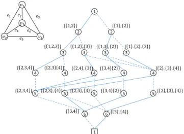
As shown in Fig. 1, we proceed by iteratively marking edges in the order given, and considering partitions of the respective elimination fronts at each level. From this figure, the width of this BDD at thek-th level, which is the number of nodes in thek-th level, is seen to be at most the number of partitions of thek-th elimination front.

Thewidth of the BDDis the maximum width over all levels. In order to use the BDD in a reasonable manner, it is necessary to keep the width of the BDD small. For example, if the width of any level becomes too large, there is the possibility that there will not be enough space available to finish the computation. We must then analyze the size of the width for our BDD-based algorithms and, in the particular case of the BDD proposed in this paper, try to find a good

Fig. 1 BDD representing all spanning trees of the complete graphK₄.

ordering of the edges so that the elimination front does not become too large.

3. BDD Representing All Spanning Trees of a Complete Graph

As described in the last Section, Sekine, Imai, Tani[2]pre- sented an algorithm to compute the BDD representing all of its spanning trees, and the following is given there.

Theorem 1([2]). For a simple, connected graph of nver- tices, the width of the BDD representing all spanning trees is bounded byBelln−2, whereBellais thea-th Bell number, the number of partitions of a set ofaelements.

In this paper we improve the bound, and obtain the following.

Theorem 2. The width of the BDD is bounded by Belln−O(n/logn).

To prove this theorem, we use a lower bound for the Bell number, which is not so tight but is enough to show our asymptotic bound.

Lemma 1. For integersa>0andb≥3, we haveBella >

b^a−b.

Proof. The remarkable formula of Dobinski [17], [18] is given by

Bella= 1 e

∞

X

j=0

j^a j!.

Considering the term where j = bin the sum above, and using the inequality

lnb!= 1 2lnb+1

2

b−1

X

i=1

(lni+ln(i+1))≤blnb−b+1+1 2lnb,

we have the lemma forb≥3.

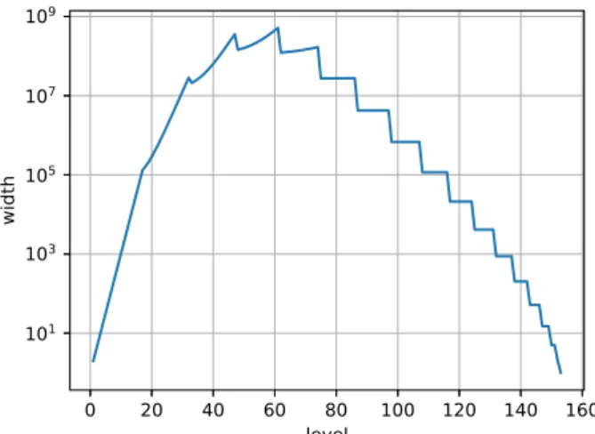
Fig. 2 Width of each level in the BDD of spanning trees of the complete graphK₁₈.

Fig. 3 Width of each level in the BDD of spanning trees of the 18×18 grid graph.

Lemma 2. For integers a ≥ 17, b := ba/lnac ≥ 6 and c:=bb/ec −1≥1, we have(c+1)^a−c+1 <Bella−c+1. Proof. From Lemma 1, we have

ln Bella−c+1

(c+1)^a−c+1 >(a−c+1)ln b

c+1−blnb

>a− a lna ln a

lna −c+1= a

lna ln lna−c+1>0 where we useb/(c+1) ≥e andb≤a/lna.

Lemma 3. For integera ≥3, f(x)=x^−x+a+2is monotoni- cally increasing forxwith2≤x≤ _{e ln}^a

a +1<_{e ln}^2a_a. Proof. (lnf(x))⁰=−lnx+(a+2)/x−1 has a single rootγ >

2. It is straightforward to check(lnf)⁰(2)and(lnf)⁰ _2a

e lna

are positive, and the lemma holds.

With the lemmas above in hands, we can prove Theo- rem 2. To facilitate understanding, we show how the width of each level of the BDD corresponding toK₁₈varies in Fig. 2.

For completeness, we also show how the width of each level of the BDD corresponding to the 18×18 grid graph varies in Fig. 3.

Proof of Theorem 2. We need only consider the case of a

complete graph K_n of n vertices, since any graph with n vertices can be obtained fromK_nby deleting edges and, thus, the size of the BDD ofK_nserves as an upper bound for the size of the BDD of the graph considered in the Theorem. As described in Sekine, Imai, Tani[2], we arbitrarily order then vertices of the graph intov₁, v₂, . . . , v_n, and then order edges ek = (v_i, v_j)with(i,j)in lexicographic order, ase₁, . . . ,e₆ in the example given in Fig. 1. We call this ordering of the edges a lexicographic edge orderingfor a given vertex ordering. Letc:=b bn/lnnc/ec −1 (this value is chosen to work well with Lemma 3 below).

For eachi∈ {1, . . . ,c}, consider the levels correspond- ing to the edges(v_i, v_i+1), . . . ,(v_i, v_n−1),(v_i, v_n). The width of the BDD does not decrease for(v_i, v_j)when j goes from i+1 ton−1, because bothv_i stays in the elimination front andv_jeither is added to it or stays in it. The width decreases for j=nbecause bothv_iandv_nare removed from the elim- ination front. Hence, for eachi ∈ {1, . . . ,c}the maximum width is attained at j =n−1. The BDD width for the level corresponding to the edges(v_i, v_n−1),i ∈ {1, . . . ,c}, can be bounded by the number of partitions of {v_i, . . . , v_n−1, v_n}, because the elimination front is contained in it. Any pair of vertices among {v_i, . . . , v_n−1, v_n}may only be contracted to the same vertex in the BDD if the edges that connect them to some v_k ∈ {v₁, . . . , v_i}are contracted. Hence the number of sets of size 2 or more in the partition is bounded by i = |{v₁, . . . , v_i}|. Sets consisting of a single vertex in the partition may be handled as a set of such single ele- ments, and then the number of partitions for{v_i, . . . , v_n}of n−i+1 elements is bounded by (i+1)ⁿ⁻ⁱ⁺¹. Therefore, for i ∈ {1, . . . ,c}, j ∈ {i +1, . . . ,n}, the width at levels corresponding to edges (v_i, v_j)is bounded by(i+1)ⁿ⁻ⁱ⁺¹, which is bounded by (c+1)^n−c+1 due to Lemma 3, which is bounded by Belln−c+1 due to Lemma 2. In summary, fori ∈ {1, . . . ,c}, j ∈ {i+1,· · ·,n}the width of the BDD with levels corresponding to the edges(v_i, v_j)is bounded by Bell_n−c+1.

Next, we consider the levels corresponding to the re- maining edges (v_i, v_j), with i ∈ {c+1, . . . ,n}, j ∈ {i + 1, . . . ,n}. For all of those levels, the verticesv₁, v₂, . . . , v_c cannot possibly be elements of the elimination front. It fol- lows that the elimination front size is at mostn−c, and the width of those levels is bounded by Belln−c. We thus obtain

the theorem.

Using a machine with memory size of 300 GB, we computed BDDs for moderately large graphs. The sizes of the obtained BDDs become as in Table 1 and Table 2.

4. FPT Algorithm with Respect to the Pathwidth Our goal in this section is to design a BDD-based FPT algo- rithm to compute all spanning trees of a graphGusing an ordering of the edges based on path decompositions ofG.

First we define (proper) interval graphs. Givenninter- vals on a line, the interval graph is their intersection graph, i.e., each interval is represented by a vertex and two vertices

Table 1 Sizes of BDDs representing all spanning trees of the complete graphKn(numbers forn=2, . . .,12 are shown in[2]), wherenandm represent the numbers of vertices and edges of the graph, respectively.

n m BDD width BDD size #(trees)

2 1 1 2 1

3 2 2 6 3

4 6 5 20 16

5 10 14 67 125

6 15 42 225 1296

7 21 130 774 16807

8 28 406 2765 262144

9 36 1266 10292 4782969

10 45 3926 39891 10⁸

11 55 15106 160837 ≈2.36×10⁹ 12 66 65232 673988≈6.20×10¹⁰ 13 78 279982 2932313≈1.79×10¹² 14 91 1191236 13227701≈5.67×10¹³ 15 105 5021562 61780185≈1.95×10¹⁵ 16 120 20983928 298329384 ≈7.21×10¹⁶ 17 136 95465291 1487514714 ≈2.86×10¹⁸ 18 153 515558869 7649388018 ≈1.21×10²⁰

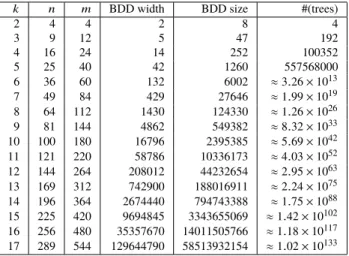
Table 2 Sizes of BDDs representing all spanning trees ofk×kgrid graphs (numbers fork = 2, . . .,12 are shown in [2]), wherenand m represent the numbers of vertices and edges of the graph, respectively.

k n m BDD width BDD size #(trees)

2 4 4 2 8 4

3 9 12 5 47 192

4 16 24 14 252 100352

5 25 40 42 1260 557568000

6 36 60 132 6002 ≈3.26×10¹³

7 49 84 429 27646 ≈1.99×10¹⁹

8 64 112 1430 124330 ≈1.26×10²⁶

9 81 144 4862 549382 ≈8.32×10³³

10 100 180 16796 2395385 ≈5.69×10⁴² 11 121 220 58786 10336173 ≈4.03×10⁵² 12 144 264 208012 44232654 ≈2.95×10⁶³ 13 169 312 742900 188016911 ≈2.24×10⁷⁵ 14 196 364 2674440 794743388 ≈1.75×10⁸⁸ 15 225 420 9694845 3343655069 ≈1.42×10¹⁰² 16 256 480 35357670 14011505766 ≈1.18×10¹¹⁷ 17 289 544 129644790 58513932154 ≈1.02×10¹³³

are connected by an edge if the two correponding intervals intersect. A proper interval graph is an interval graph where no interval properly contains another interval[19].

The pathwidth of a graph can be characterized by inter- val graphs[20]. Theorem 29 in the last reference states that, for a graphG, the pathwidth ofGis at mostk−1 if and only if interval thickness is at mostk, where the interval thickness ofGis the smallest maximum clique size of an interval graph containingGas its subgraph. The proper pathwidth ofGis defined by restricting the interval graph to a proper interval graph.

Proposition 1. For any graphGofn vertices, there exists an ordering of the edges in which the size of the elimination front is bounded bypw(G)+1.

Proof. As discussed above, there exists an interval graph ofn intervals with maximum clique of size pw(G)+1, and with endpoints having different coordinates {1,2, . . . ,2n}. Fur- thermore, this graph containsGas a subgraph, thus a bound

on the size of its elimination front implies a bound on the size of the elimination front ofG. We initially order its vertices in increasing order of their right endpoints. Using this vertex orderingv₁, . . . , v_n, we order the edges in the lexicographic order, obtaining an edge orderinge₁,e₂, . . . ,e_m. Consider an arbitrary levelkcorresponding to the edgee_k =(v_m, v_n), m < n, in the BDD of this interval graph. From the way we ordered the edges, we can say that (i) all the edges e_i adjacent to a vertex in{v₁, . . . , v_m−1}are such thati ≤k; (ii) all the edgese_i =(v_p, v_q), wherem < p <qare such that ei >k. It follows that all the vertices in the elimination front are adjacent tov_m(or equal tov_m), and thus the size of the elimination front is bounded by the maximum clique size of

the interval graph, i.e. pw(G)+1.

Proposition 2. For any graphG, there exists an ordering of the edges in which the size of the elimination front is bounded byppw(G).

Proof. By an argument similar to the one in the proof of the proposition above, we need only consider the case of a graph which is a proper interval graph with maximum clique size ppw(G) (containingGas a subgraph). We again use the lexicographic edge ordering as above. For a vertexv, let I(v)denote its corresponding interval. Consider an arbitrary levelkcorresponding to the edgee_k =(v_i, v_j),i< j, in the BDD of this interval graph. Letv_i(1), . . . , v_i(k)(in increasing order) be vertices whose intervals intersect with the right endpoint of I(v_i). Due to the properness of the interval graph, v_i(k) cannot be on the elimination front, so its size is at most ppw(G). When the edge(v_i, v_i(k)) is searched, the elimination front containsv_i(k), but does not containv_i anymore (we call this situationgood). Thus, this elimination

front has size at most ppw(G).

It should be noted that if a general interval graph G necessarily encounters a good situation, its elimination front size becomes bounded by pw(G).

Now we are ready to use the theorem below to bound the width of the BDD of our algorithms.

Theorem 3(Sekine, Imai, Tani[2]). Let`be the maximum size of the elimination front for a given edge ordering. Then, the width of the BDD of all spanning trees of G by the partition isomorphism is bounded byBell`.

Corollary 1. Given a graph G with its (proper) interval graph representation of interval thicknesspw(ppw, respec- tively), we can compute an edge ordering such that the max- imum size of elimination front ismin{pw+1,ppw}and the BDD width is bounded byBellmin{pw+1,ppw}.

Here we describe some examples. For two integersh and k with h ≤ k consider an h×k grid graph with hk vertices and 2hk−k−hedges. The pathwidth of the grid graph ish(e.g., see[20]), and it can be seen that the proper pathwidth is alsoh. Hence, the elimination front size can be bounded byh.

We can also consider ah×k×lthree-dimensional grid

graph, for integersh ≤ k ≤ l. It has been proven that, in the general case, the bandwidth of such a graph equals its pathwidth[21]. But it is also known that the bandwidth of any graph coincides with their proper pathwidth, and the size of its elimination front can be bounded byhkifh+k−2≤l, andhk− b(h+k−l−1)²/4cotherwise[22].

The (two-dimensional) grid graph is planar, which makes the number of possible partitions on the elimination front smaller than the Bell number[2], and the BDD width isC_h, whereC_his theh-th Catalan number. In Table 2, for eachk=2, . . . ,17 the width of the BDD of the square grid graph is equal toC_k.

5. Connection with Separator Theorems

We note here that the relationship between treewidth, path- width and separators is well known. A graph with treewidth tw has a separator of size tw, but the opposite does not hold necesarily[23]. Furthermore, a graph with pathwidth pw has a separator of size pw, and additionally if the size of the separator is given byO(n^σ), for someσwith 0< σ <1, (re- spectivelyO(1)), the pathwidth equalsO(n^σ)(respectively O(log(n))).

The planar separation theorem, cited in the introduc- tion, has been extended to wider classes of graphs by many researchers (e.g., [24]), and Kawarabayashi and Reed[22]

showed that ann-vertex graph with no K_t-minor for some integer t has a 2/3-separator of size O(t√

n), and further showed and sketched that this separator can be found in O(n²)andO(n¹⁺)time, respectively, for any >0. They also showed that for ann-vertex planar graph there is a good edge ordering, computable inO(nlogn)time, such that the size of the elimination front isO(√

n). Applying the same arguments, it can be shown that for ann-vertex graph with no Kt-minor, there is an edge ordering, computable inO(n⁰) time for any⁰>0.

Graphs having nice separators are known in a class of geometric graphs, such as sphere-packing graphs[25], finite element meshes[26], string graphs[27].

6. Conclusion

In this paper, we revisit an earlier BDD-based algorithm to enumerate spanning trees and compute Tutte polynomials of graphs, and improve previous bounds on the the width of the BDD generated by it. We further propose an FPT alternative of this algorithm, based on the path decomposition of the graphs.

Acknowledgments

This work was supported by JSPS KAKENHI Grant Num- bers 15H01677, 16K12392, 17K12639. We thank the two anonymous reviewers for their constructive comments and suggestions.

References

[1] R.E. Bryant, “Graph-based algorithms for boolean function manip- ulation,” IEEE Trans. Comput., vol.35, no.8, pp.677–691, 1986.

[2] K. Sekine, H. Imai, and S. Tani, “Computing the Tutte polynomial of a graph of moderate size,” Algorithms and Computations, Lecture Notes in Computer Science, vol.1004, pp.224–233, Springer Berlin Heidelberg, 1995.

[3] R.J. Lipton and R.E. Tarjan, “A separator theorem for planar graphs,”

SIAM J. Appl. Math., vol.36, no.2, pp.177–189, 1979.

[4] W.T. Tutte, “A contribution to the theory of chromatic polynomials,”

Canad. J. Math., vol.6, pp.80–91, 1954.

[5] D.L. Vertigan and D.J.A. Welsh, “The computational complexity of the Tutte plane: The bipartite case,” Combinator, Probability and Computing, vol.1, no.2, pp.181–187, 1992.

[6] D.J.A. Welsh, Complexity: Knots, Colourings and Counting, Cam- bridge University Press, New York, NY, USA, 1993.

[7] F. Jaeger, D.L. Vertigan, and D.J.A. Welsh, “On the computational complexity of the Jones and Tutte polynomials,” Math. Proc. Cam- bridge Phil. Soc., vol.108, no.1, pp.35–53, 1990.

[8] H. Imai, S. Iwata, K. Sekine, and K. Yoshida, “Combinatorial and ge- ometric approaches to counting problems on linear matroids, graphic arrangements, and partial orders,” Computing and Combinatorics, Lecture Notes in Computer Science, vol.1090, pp.68–80, Springer Berlin Heidelberg, 1996.

[9] K. Sekine, H. Imai, and K. Imai, “Computation of the Jones polyno- mial,” Trans. Japan Society for Industrial and Applied Mathematics, vol.8, no.3, pp.341–354, 1998 (in japanese).

[10] H. Imai, K. Sekine, and K. Imai, “Computational investigations of all- terminal network reliability via BDDs,” IEICE Trans. Fundamentals, vol.E82-A, no.5, pp.714–721, May 1999.

[11] H. Imai, “Computing the invariant polynomials of graphs, networks and matroids,” IEICE Trans. Inf. & Syst., vol.E83-D, no.3, pp.330–

343, March 2000.

[12] D.E. Knuth, The Art of Computer Programming, Volume 4, Fas- cicle 1: Bitwise Tricks & Techniques; Binary Decision Diagrams, 12th ed., Addison-Wesley Professional, 2009.

[13] S. Minato, “Zero-suppressed BDDs for set manipulation in com- binatorial problems,” Proc. 30th International Design Automation Conference, pp.272–277, ACM, 1993.

[14] N. Robertson and P.D. Seymour, “Graph minors. I. Excluding a forest,” J. Comb. Theory, Ser. B, vol.35, no.1, pp.39–61, 1983.

[15] R.G. Downey and M.R. Fellows, Parameterized Complexity, Springer, 1999.

[16] R.E. Bryant, “Symbolic Boolean manipulation with ordered binary- decision diagrams,” ACM Comput. Surv., vol.24, no.3, pp.293–318, 1992.

[17] G. Dobinski, “Summierung der reihe P∞

n=1n^m/n! für m =

1,2, . . .,” Arch. für Mat. und Physik, vol.61, pp.333–336, 1877.

[18] G.C. Rota, “The number of partitions of a set,” The American Math- ematical Monthly, vol.71, no.5, pp.498–504, 1964.

[19] H. Kaplan and R. Shamir, “Pathwidth, bandwidth, and completion problems to proper interval graphs with small cliques,” SIAM J.

Comput., vol.25, no.3, pp.540–561, 1996.

[20] H.L. Bodlaender, “A partialk-arboretum of graphs with bounded treewidth,” Theor. Comput. Sci., vol.209, no.1-2, pp.1–45, 1998.

[21] Y. Otachi and R. Suda, “Bandwidth and pathwidth of three- dimensional grids,” Discrete Math., vol.311, no.10, pp.881–887, 2011.

[22] K. Kawarabayashi and B. Reed, “A separator theorem in minor-closed classes,” Proc. 2010 IEEE 51st Annual Symposium on Foundations of Computer Science, FOCS ’10, pp.153–162, IEEE Computer So- ciety, 2010.

[23] B.A. Reed, “Finding approximate separators and computing tree width quickly,” Proc. Twenty-fourth Annual ACM Symposium on Theory of Computing, STOC’92, pp.221–228, ACM, 1992.

[24] N. Alon, P. Seymour, and R. Thomas, “A separator theorem for graphs with an excluded minor and its applications,” Proc. Twenty-second Annual ACM Symposium on Theory of Computing, STOC’90, pp.293–299, ACM, 1990.

[25] G.L. Miller, S.H. Teng, W. Thurston, and S.A. Vavasis, “Separators for sphere-packings and nearest neighbor graphs,” J. ACM, vol.44, no.1, pp.1–29, Jan. 1997.

[26] G. Miller, S. Teng, W. Thurston, and S. Vavasis, “Geometric separa- tors for finite-element meshes,” SIAM J. Sci. Comput., vol.19, no.2, pp.364–386, 1998.

[27] J. Matoušek, “Near-optimal separators in string graphs,” Combinator.

Probab. Comput., vol.23, no.1, pp.135–139, 2014.

Farley Soares Oliveira received his asso- ciate’s degree from the Department of Informa- tion Engineering, National Institute of Technol- ogy, Nara College in 2016 and his bachelor’s degree from the College of Information Science, School of Informatics, University of Tsukuba in 2018. He is currently working towards a master’s degree at the Department of Computer Science, University of Tokyo.

Hidefumi Hiraishi received Ph.D. from Department of Computer Science, University of Tokyo in 2016. He is an assistant professor of Department of Computer Science, University of Tokyo. His research interests include matroid theory, combinatorial optimization and quantum computation.

Hiroshi Imai B. Eng. and D. Eng. from the University of Tokyo, 1981 and 1986, respec- tively. Associate Professor at Kyushu University from 1986, moved to the University of Tokyo in 1990, and now a professor in computer science there. JST ERATO Quantum Computation and Information Project Leader during 2000–2011.