JAIST Repository: A controllable model of a random multiplicative process for the entire distribution of population

全文

(1)JAIST Repository https://dspace.jaist.ac.jp/. Title. A controllable model of a random multiplicative process for the entire distribution of population. Author(s). Tomita, Shinji; Hayashi, Yukio. Citation. Physica A: Statistical Mechanics and its Applications, 387: 1345-1351. Issue Date. 2008-02-15. Type. Journal Article. Text version. author. URL. http://hdl.handle.net/10119/7914. Rights. NOTICE: This is the author's version of a work accepted for publication by Elsevier. Shinji Tomita, Yukio Hayashi, Physica A: Statistical Mechanics and its Applications, 387, 2008, 13451351, http://dx.doi.org/10.1016/j.physa.2007.09.028. Description. Japan Advanced Institute of Science and Technology.

(2) A Controllable Model of Random Multiplicative Process for Entire Distribution of Population Shinji Tomita ∗ and Yukio Hayashi School of Knowledge Science, Japan Advanced Institute of Science and Technology 1-1 Asahidai, Nomi-city, Ishikawa 923-1292. Abstract A random multiplicative process (RMP) is one of the basic models which can generate a power law distribution. Actually, the distribution generated by RMP has two parts, which are closely matched to the head of a lognormal distribution and the tail of a power law distribution. We investigated the relation between a shape of distributions and model variables. By changing input variables, we explained the origin of the cumulative population distributions of municipalities and prefectures in Japan from 1980 to 2006. This controllability of RMP can be applied to a power law distribution in various other fields. Keywords: Random Multiplicative Process; controllability; cumulative population distribution;. 1.. Introduction The evolution of the population seems to change with time due to various factors such as economy,. environment and policy, etc. However, there is empirical regularity about the distribution of the population. Zipf ’s law for cities is one of the most striking empirical facts. Zipf ’s law: In terms of distribution, this means that the probability that the size of a city is greater than some S is approximately proportional to 1/S. N(Size ≥ S) = aS -β with β ≅ 1 in general. Zipf ’s law holds across countries with very different economic structures and histories such as the early and modern United States [1], France and Japan in the twentieth century [2], China in the mid-nineteenth century [3], and India in the early twentieth century [4]. Though this law seems to be robust, in previous literature on Zipf ’s law, only large cities were considered [5]. This implies that most samples of small cities were ignored. However, when we think about entire distribution of population, we cannot ignore small cities. Actually, in the high growth of the Japanese economy after 1955 a great demographic shift happened, since the young persons migrated to the city regions from the rural regions. Forty percent of municipalities are specified as depopulated areas now. We can’t see the entire problem by considering only large cities. Therefore, the entire distribution of population and its generation mechanism should be studied. The purpose of this paper is twofold. First, we explain the cumulative population distributions of (all) municipalities and prefectures in Japan. Second, we investigate the origin of those distributions by a random multiplicative process (RMP), which is a simple model. We show that the real data of cumulative population distribution are almost constant, and this data can be generated by controlling variables of the RMP. The organization of this paper is as follows. In the next section, we analyze the cumulative population distribution of all municipalities and prefectures in Japan from 1980 to 2006. In Section 3, we introduce the RMP. In Section 4, we examine the features of the distribution generated by the RMP. In Section 5, we fit simulated results with real data. In Section 6, we ∗. Corresponding author.. E-mail addresses: [email protected] (Shinji Tomita), [email protected] (Yukio Hayashi).

(3) summarize our results. 2.. Data analysis We have a total population of 127.92 million in Japan at present. The population in 2006 was the. tenth largest in the world, equivalent to 2.0 percent of the global total 1 . This population occupies over 1800 municipalities and 47 prefectures. In this paper, we treat two kinds of data. The first is population of municipalities (micro scale) and second is prefectures (medium scale). We analyze the distribution of population in the range from micro-scale aspect and medium-scale one, and investigate the common features. We acquired the data of municipalities 2 and prefectures 3 from the Statistics Bureau in Japan. The main advantage of using these census data is that they cover the entire population distribution. Municipality is a generic name for a city, a town, or a village. Most municipalities have very few inhabitants. A number of municipalities have been eliminated after a great merge in 2000. Table 1 shows transition of number of municipalities; the total number of municipalities has decreased by 1435 in these 26 years. Table.1 Number of Municipalities Year Number of municipalities. 1980. 1985. 1990. 1995. 2000. 2006. 3257. 3253. 3253. 3234. 3229. 1822. Number of eliminated municipalities. -4. 0. -19. -5. -1407. A prefecture consists of a larger area including municipalities (cities, towns, and villages). The number of prefectures has been 47 for a long time. Figure 1 shows the cumulative population distributions of municipalities (a) and of prefectures (b), respectively. From these figures, the entire distribution seems not to have changed so much in these 26 years. The distributions seem to be divided into upper part (upper 20%) and lower part (lower 80%), both on a micro scale (municipalities) and a medium scale (prefectures). The upper parts of the distributions of municipalities and prefectures correspond to over 30000 and 4000000 inhabitants. This means that the distribution deviates from a power law in the lower 80% part. We call the lower 80% part of the distribution the “head”, and the upper 20% part the “tail”. These two parts are similar to the double Pareto distribution, which is closely matched to the head of a lognormal distribution and the tail of a power law distribution [6]. In the tail part, a power law can be expressed as. N ( x) = ax − β. (1). where N(x) and x are the rank of a site (municipality or prefecture) and the population, respectively.. β denotes an exponent in the power law. By taking logarithm, Eq.(1) is rewritten as. ln N ( x) = ln a − β ln x. (2). After calculating a regression expression in the tail part by least squares method, the exponent of. 1 2. 3. http://memorva.jp/ranking/unfpa/who_2006_population.php Data of 1980, 85, 90, 95 and 2000: http://www.stat.go.jp/data/kokusei/2000/kako/danjo/index.htm 2006: http://www.soumu.go.jp/c-gyousei/020918.htm Data of 1980, 85, 90 and 95: http://www.stat.go.jp/data/jinsui/wagakuni/index.htm 2000: http://www.stat.go.jp/data/jinsui/2-3.htm 2006: http://www.soumu.go.jp/c-gyousei/020918.html.

(4) municipalities is 1.19 ± 0.04, and the exponent of prefectures is 2.49 ± 0.06. It can be said that these distributions are stationary states. (a). (b). 104. Municipality 1980 1985 1990 1995 2000 2006. 103. 10. head N(x). N(x). head. 2. 10. 2. Prefecture 1980 1985 1990 1995 2000 2006. 1. 10. tail 101. tail 10. 0. 10. 0. 2. 10. 3. 4. 5. 10. 10. 6. 10. 7. 10. 10. 6. 7. 10. x. 10 x. Fig. 1. Log-log plots of the rank of the site N(x) vs. the population x from 1980 to 2006. (a) municipalities and (b) prefectures. The solid lines are power laws with the exponents 1.2 (a) and 2.5 (b), respectively. Dotted lines are the diverging point of head (lower 80%) and tail (upper 20%).. 3.. The controllable model We consider a Random Multiplicative Process (RMP) proposed by Takayasu [7, 8] to generate the. real population distributions of municipalities and prefectures. The RMP is one of the basic models which can generate a power law distribution in the upper tail. The fundamental idea of the RMP was pointed out by Champernowne [9], and the mathematical formalization is given by Kesten [10]. The RMP is a stochastic process with multiplicative and additive noises. The model equation is characterized by the following stochastic time evolution equation:. xi (t + 1) = bi (t ) xi (t ) + f i (t ). i = 1,2,...N. (3). where xi(t) denotes the population of the i-th municipality or prefecture at time t. bi(t) > 0 is a multiplicative noise; xi(t+1) increases for bi(t) > 1 and decreases for bi(t) < 1, and fi(t) is an additive noise. Takayasu set the distribution functions of bi(t) and fi(t) according to the Poisson distribution and the symmetric Gaussian, respectively. However, the result of a power law distribution doesn’t depend on these or any other settings [11]. In other words, we can obtain it from any kind of distribution. In the context of population dynamics, bi(t) and fi(t) can be interpreted as the growth rate and unexpected comings and goings, respectively. Because these noises include various factors, it is difficult to specify the explicit distribution form. A further argument is necessary to specify the physical meanings of noise. For the sake of simplicity, we assume bi(t) and fi(t) are generated by uniformly random noises in a certain range, independent of time, temporarily. There are two reasons that we assume bi(t) and fi(t) to be uniformly random noises in a certain range. First is that growth rate bi(t) and unexpected comings and goings fi(t) will be bounded variables, not infinite. Second is that uniform distribution may include various cases, because it does not assume specified distribution. We should remark that random multiplicative noise bi(t) corresponds to growth rate, which does.

(5) not depend on the size of the sites . This is confirmed in the United States [12] and Japan [13]. All cities follow similar processes; i.e., their growth processes have a common mean (equal to the mean city growth rate). This homogeneity of growth processes is often referred to as Gibrat’s law [14]. The RMP can generate a power law distribution with the specified exponent β. The relationship between exponent β and multiplicative noise b(t) is given by the expectation. bβ = 1. (4). This relation leads to the following expression.. 1 bmax − bmin. ∫. bmax bmin. b β db = 1. (5). where bmax and bmin are the upper and lower limits of multiplicative noise b(t), respectively. Figure 2 illustrates the method of deciding the range of multiplicative noise b(t). The areas of ① and ② are equal. For examples, we obtain bmin = 0.24 and baverage = 0.92 by calculation from Eq.(5) after setting β = 2.0 and bmax = 1.6. If bmax decreases, range of b(t) narrows and baverage increases. Conversely, if bmax increases, range of b(t) widens and baverage decreases. From these relations between range of b(t) and. baverage, after this, we focus on baverage. 4 3.5 3. bβ. 2.5 2 1.5. ②. 1. ①. 0.5 0 0. bmin. 0.5. 1. 1.5. bmax. 2. b. Fig. 2. Method of deciding range of multiplicative noise b(t). The random variable b(t) is generated by a uniform random number within range [bmin ,bmax].. 4.. The relationship between variables and distribution Before fitting the model with the real data, we examined the features of the distribution generated. by the RMP. First, we investigated the relationship between noise and shift of distribution. We set β = 2.5, baverage = 0.99, frange = 1 and number of sites = 1000, respectively. Figure 3 shows the relationship between additive noise f(t) and shift of distribution. We can shift the distribution to the right by increasing either faverage or baverage. Similarly, we can shift it to the left by decreasing either faverage or. baverage..

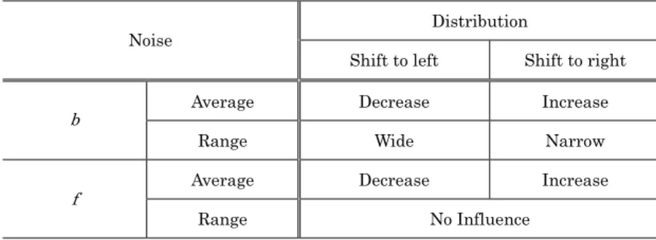
(6) 10. 3. 10. 2. N(x). 4000 20000 40000. 101. 10. 0. 10. 4. 10. 5. 10 x. 6. 10. 7. 8. 10. Fig. 3. The relationship between additive noise f (t) and shift of distribution. Each symbol stands for faverage; (○) = 4000, (☓) = 20000, (□) = 40000. The relationship between noise and shift of distribution is summarized in Table 2. When we fix. baverage and want to shift the distribution to the left, we should decrease faverage. Conversely, when we fix baverage and want to shift the distribution to the right, we should increase faverage. Decreasing baverage corresponds to widening brange. Increasing baverage corresponds to narrowing brange. When we fix faverage and want to shift the distribution to the left, we should decrease baverage. Conversely, when we fix faverage and want to shift the distribution to the right, we should increase baverage. We confirmed that the stationary distribution does not depend on the value of frange.. Table 2. The relationship between noise and shift of distribution Distribution. Noise. b. f. Shift to left. Shift to right. Average. Decrease. Increase. Range. Wide. Narrow. Average. Decrease. Increase. Range. No Influence. Next, we investigated the relationship between the number of sites and the distribution range. Figure 4 shows the cumulative distributions according to the number of sites. We can expand the distribution by increasing the number of sites. Especially, head and tail are expanded by increasing the number of sites. The distribution range of municipalities is wide, because the number of municipalities is very large (over 1600). On the other hand, the distribution range of prefectures is narrow, because the number of prefectures is very small (47)..

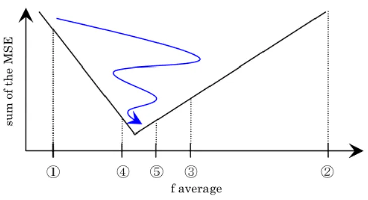
(7) 10. 4. 100 1000 10000. N(x). 103. 10. 2. 10. 1. 10. 0. 10. 5. 10. 6. 10 x. 7. 10. 8. 9. 10. Fig. 4. The relationship between the number of sites and the distribution range. Log-log plots for the cumulative population distribution. Each symbol stands for number of sites; (○) = 100, (☓) = 1000, (□) = 10000.. From examining the features of the RMP, we can control the shift of distribution, which depends on the values of additive noise f(t) and multiplicative noise b(t), and we can control the distribution range, which depends on the number of sites.. 5.. The data fitting To fit the model with the real data, we search appropriate variables systematically by applying a. binary search. Though specific distribution can be generated just by controlling one noise, additive noise f(t) or multiplicative noise b(t), here, we set β, baverage and number of sites respectively, and search for faverage. As a procedure, we repeat RMP → Compare sum of the mean squared errors (MSE) of real data and simulated result → RMP…, until we arrive at an appropriate faverage. Figure 5 shows. sum of the MSE. procedure of search for faverage.. ①. ④. ⑤. ③. ②. f average. Fig. 5. Procedure of search for faverage. When faverage approaches the appropriate value, sum of MSE decreases..

(8) Procedure of search for faverage is as follows,. Step 1. Chose an initial very small faverage ① as the minimum initial value, and calculate a regression expression in the tail part of simulated result. Calculate the following sum of the MSE between the real data and simulated result on the approximation line. Sum of the MSE is as follows,. S e = ∑ ( yreal − ysim ). 2. (6). where yreal and ysim are rank of the site on approximation lines of real data and simulated result, respectively. Step 2. Chose very large faverage ② as the maximum initial value and calculate the sum of the MSE, the same as in Step 1. Step 3. Chose middle point ③ of ① and ②. Step 4. Compare sum of the MSE ① and ②, If ①’s error is smaller than ②’s, chose middle point ④ of ① and ③. Step 5. Compare sum of the MSE ① and ③, If ③’s error is smaller ①’s, chose middle point ⑤ of ③ and ④… Step 6. When the shift value of faverage becomes less than 1, these processes are stopped.. Fitting the simulated result with the real data First, we investigated fitting the simulated result with two points of municipalities’ real data (1980 and 2006), because the number of municipalities has decreased greatly in this period. For 1980 data, we set β = 1.16, baverage = 0.99 and number of sites = 3257, respectively, and searched for faverage corresponding to these constants. We obtained faverage as 67.62, sum of MSE as 930000.1, and MSE as 1.49. For 2006 data, we set β = 1.31, baverage = 0.99, and number of sites = 1822, respectively, and obtained faverage as 215.70, sum of MSE as 174322.2, and MSE as 1.15. Similarly, we fitted simulated result with the average of prefectures real data from 1980 to 2006. We set β = 2.49, baverage = 0.99 and number of sites = 47, respectively, and obtained faverage as 34763.9, sum of MSE as 2.44, and MSE as 0.17. In Figure 6, not only the approximation line of simulated result and real data, but also the whole distributions, overlap almost completely. These results show the simulated results generated by the RMP and the real data are in very good agreement..

(9) (b). 104. 10. 3. 10. 2. 10. 1. 10. 0. 102. 1980 real sim. 104. 2006 real sim. N(x). N(x). (a). 103. Prefecture real sim. 101. 102 101 100 102. 2. 10. 103. 3. 10. 104. 105. 10. 106. 4. 107. 105. 106. 107. 100. 6. 7. 10. 10. x. x. Fig. 6. Log-log plots of the rank of the sites N(x) vs. the population x from 1980 to 2006; (a) municipalities and (b) prefectures. The solid lines and dotted lines represent the approximation lines of real data and simulated result, respectively. Symbol (○) and (☓) stand for real data and simulated result, respectively.. Trade-off relationship between variables In the previous subsection, we searched for faverage in the setting of β, baverage and number of sites. However essentially, even if one variable is fixed or changed, specified distribution can be generated by the RMP. baverage is on trade-off relations with faverage. Here, we research the trade-off relation between. baverage and faverage when distribution of municipalities in 2006 is generated. Figure 7 shows the relationship between baverage and faverage. It is obvious that baverage is proportional to faverage. Because bi(t) is a non dimensional variable (growth rate) and fi(t) is a dimensional variable (number of people), those scales are different. When the average of the growth rate (baverage) is small, large faverage is necessary to reproduce the population distribution of Japan. On the contrary, faverage may be small, when the average of the growth rate (baverage) is large.. This implies that there are many combinations of noises. which can reproduce real population distribution. One of these combinations might correspond to the noise of the real world. It will be a further study to estimate what kinds of combinations are realistic. 6000 5000. f average. 4000 3000 2000 1000 0 0.94. 0.95. 0.96. 0.97 0.98 b average. 0.99. Fig. 7. The relationship between baverage and faverage.. 1.

(10) 6.. Concluding Remarks In summary, we have investigated the cumulative population distribution of all sites. (municipalities and prefectures) in Japan from 1980 to 2006, and they seem not to have changed so much in these 26 years. Especially, the exponent in tail part (β ) has hardly changed. This appears similar to the double Pareto distribution, which is closely matched to the head of a lognormal distribution, and the tail of a power law distribution. We reproduced these distributions by the RMP which combined two kinds of noises recursively. In the RMP, we indicated that the entire distribution of population can be reproduced by using the exponent in tail part. It is very interesting to be able to reproduce the population distribution by such a simple mechanism. Additionally, we clarified the features of the distribution generated by the RMP under noise control. Multiplicative noise baverage is on trade-off relations with additive noise faverage. The controllability by changing noises can be applied to a power law distribution in various other fields. For future work, we should investigate the social meaning of noises. Specifying the meaning of these noises and knowing methods to control them may be very useful for planning various policies.. Reference [1]. E. Glaeser, J. Scheinkman, and A. Shleifer, “Economic Growth in a Cross-Section of Cities,” Journal of Monetary Economics, XXXVI, 117-143, 1995.. [2]. J. Eaton and Z. Eckstein, “Cities and Growth: Theory and Evidence from France and Japan,” Regional Science and Urban Economics, 27(4-5), pp. 443-474, 1997. [3]. G. Rozman, “East Asian Urbanization in the Nineteenth Century,” in Van der Woude et al., pp. 61-73, 1990.. [4]. G. Zipf, “Human Behavior and the Principle of Least Effort,” Cambridge, MA: Addison-Wesley, 1949.. [5]. X. Gabaix, “Zipf ’s Law for Cities: An Explanation,” The Quarterly Journal of Economics, vol. 113, no. 3 (August), pp.739-767, 1999. [6]. M. Mitzenmacher, “Dynamic Models for File Sizes and Double Pareto Distributions,” Internet Mathematics Vol. I, No. 3: 305-333, 2003. [7]. H. Takayasu, A. Sato and M. Takayasu, “Stable Infinite Variance Fluctuations in Randomly Amplified Langevin Systems,” Phys. Rev. Lett. 79, 966, 1997. [8]. A. Sato, “Explanation of power law behavior of autoregressive conditional duration processes based on the random multiplicative process,” Phys. Rev. E 69, 047101, 2004. [9]. D. G. Champernowne, “A Model of Income Distribution,” Economic Journal, 63(250), pp. 318-475, 1953.. [10] H. Kesten, “Random Difference Equations and Renewal Theory for Products of Random.

(11) Matrices,” Acta Mathematica, CXXI 207-248, 1973. [11] S. C. Manrubia and D. H. Zanette. “Stochastic multiplicative processes with reset events,” Phys. Rev. E, vol. 59, pp. 4945-4948, 1999. [12] J. Eeckout. “Gibrat’s Law for (All) Cities,” AMERICAN ECONOMIC REVIEW, VOL. 94, NO.5, 1429-1451, 2004. [13] Y. Sasaki, H. Kuninaka, N. Kobayashi and M. Matsushita, “Characteristics of Population Distributions in Municipalities,” J. Phys. Soc. Jpn., Vol. 76, No. 7, 2007. [14] R. Gibrat, “Les inégalités économiques (Economic Inequalities),” Paris, France: Librairie du Recueil Sirey, 1931..

(12)