A Simple Option Pricing Model with Markovian Volatilities

Journal of the Operations Research Society of Japan

Vol. 36, No. 3, September 1993

A SIMPLE OPTION PRICING MODEL

WITH MARKOVIAN VOLATILITIES

Masaaki Kijima Toshihiro Yoshida

University of Tsukuba, Tokyo Sa/omon Brothers Asia Limited

(Received October 8, 1992; Revised April 28, 1993)

Abstract This paper develops a stochastic volatility model, which overcomes the Black-Scholes model tendency to overprice near at-the-money options and underprice deep out Or in-the-money options. In contrast to the previous literature that assumes diffusion volatilities, this paper assumes that the volatility follows a Markov chain on a discrete state space. This intuitive approach has easier mathematics and, by taking limit, the diffusion results can be obtained. By generalizing the binomial model to the Markovian volatility model, a refursive pricing scheme is first developed, under a particular assumption on prefer.ence to the volatility dynamics, and then a continuous time result by taking limit. The both discrete and continuous models give general conditions under which the call value is increasing in the current volatility. Also. based on the local convexity and concavity of thp Black-Scholes equation in volatility, we explain why the deficits of the Black-Scholes equation take place. Some numerical experiments are also given to support our results.

1 Introduction

Black and Scholes (BS) equation [2] has been widely recognized as a useful tool to deter-mine the price of a call option written on a stock whose price fluctuation obeys a geometric Brownian motion process. Despite of the questionable Brownian motion assumption, the very reason that the BS equation is so widely used is its easily computable form. How-ever, it has been pointed out that the BS equation involves problems that are intolerable for practitioners (see, e.g., Rubinstein [26]). For example, the BS equation works poorly (underprices) for deep out or in-the-money options whereas it overprices near at-the-money options (see, e.g., Finnerty [9] and MacBeth and Merville [20]). A natural way to overcome such deficits of the BS equation is to construct CL model that allows for the volatility of stock

returns to change over time, since the volatility is the only parameter taken from stock prices into the BS equation, and also since there is some empirical evidence that indicates that the volatility does ch angel .

Since 1987, many papers concerning option pricing with stochastic volatility have been published, most of which assume that the volatility follows a diffusion process2• For

exam-ple, Hull and White [15] and Wiggins [30] use a geometric Brownian motion as the volatility dynamics, Scott [27] and Stein and Stein [28] an Ornstein- Uhlenbeck process, whereas John-son and Shanno [17], Bailey and Stulz [1] and Heston [13] assume a square root process (see, e.g., Cox, Ingersoll and Ross [6]) or its slight generalization3_{. Since, in those models, there} 1 Another way to do this may be to use a fat-tailed process as the stock price process. Assuming Naik

and Lee's equilibrium pricing [24], Madan and Milne [21] derive an approximate call option price when the variance Gamma (VG) process [22] is used as the uncertainty driving the stock price, and compare it with the BS price. They conclude through numerical experiences that VG values are typically higher than BS values especially for out-of-the-money options.

2Follmer and Scltweizer [10] consider a very general model and develop a pricing scheme for contingent claims in an incomplete market by a remaining-risk-minimization strategy.

3 As Bailey and Stulz [1] point out, the economic relevance of stochastic volatility option models depends

150 M. Kijima & T Yoshida

are two assets in the market consisting of one risky stock and one riskless bond and since volatility is not a traded asset, the market is incomplete so that options written on the stock can not be priced by the usual arbitrage arguments (see, e.g., Harrison and Pliska [12]). In order to price such contingem claims, we need to determine the "price of volatility risk". Wiggins [30] uses an intertemporal general equilibrium model of Cox, Ingersoll and Ross [5] and shows that the case of a representative investor with log-utility leads to the price of volatility risk being zero, where the option is assumed to be written on a market portfolio whose price process is uncorrelated to the volatility process (see also Stein and Stein [28]). Heston [13] makes a particular assumption on the price of volatility risk while Bailey and Stulz [1] relate the volatility dynamics to the interest rate dynamics and then make use of a result of Cox, Ingersoll and Ross [6]. Hull and White [15] and others assume that investors' attitude to volatility risk is ne':1tral, i.e., the price of volatility risk is a priori assumed to be zero. Each of these assumptions is sufficient to price all contingent claims and they obtain respective partial differential equations which option pricing must satisfy. Furthermore, for the case that the stock price process and the volatility dynamics are independent of each other, Hull and White [15] and Scott [27] show that the solution is given as an integral of the BS equation with respect to the distribution function of the volatility dynamics. Therefore, in principle, the option price can be evaluated numerically. Unfortunately, however, these formulas are very difficult to compute so that they ought to go into either approximations or Monte Carlo simulation. Although they found through extensive numerical works that the stochastic volatility models are better at explaining actual option prices, the computational difficulty often makes the models impractical.

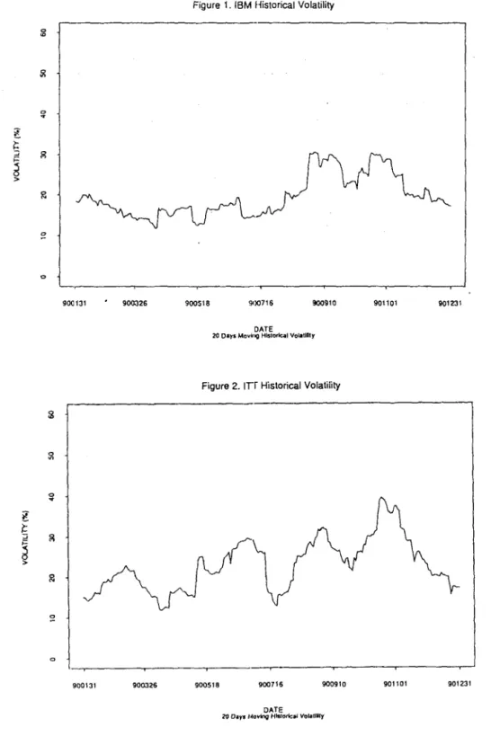
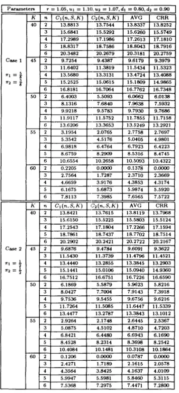
On the other hand, from the points of view of model construction, it is unclear why the volatility dynamics should have a continuous path. For example, many practitioners feel that there are two situations, in one of which a stock price fluctuates up and down quickly and in the other its movement is relatively slow. The two cases, of course, correspond to the situations of high volatility and of low volatility, respectively. In Figure 1, we plotted historical volatilities of daily returns on IBM during 1990, where volatility values are cal-culated as a moving standard deviation of 20 days. It can be observed that the periods before September and after November have a low level of volatility and the other a high volatility. Although, more generally, we may need to assume multi-levels of volatility\ a discrete model is attractive because of the following reasons: First, under some regularity conditions, many continuous models can be obtained as limits of the corresponding discrete models. Second, discrete models can describe our intuitions behind more directly, and third, the mathematics used is usually more elementary and transparent. In this paper, assuming that the volatility dynamics follows a Markov chain on a discrete state space, we construct a simple stochastic volatility model and derive an option pricing scheme.

This paper is organized as follows. In the next section, we develop a discrete-time model in which the stochastic law of volatility is described in terms of a discrete-time Markov chain. This model can be regarded as an extension of the binomial model of Cox, Ross and Rubinstein [7]. Under a particular assumption on preference to the volatility dynamics, a recursive pricing scheme is developed for European call options. Based on this formula, we then show that, if the underlying Markov chain is stochastically monotone, the higher current volatility the higher the option price. This conclusion affirms a well recognized phenomenon in actual option prices. In Section 3, we then derive a continuous-time model by shrinking both the size of movement of the stock price and the time scale at the same time, but not the state of volatility. The continuous-time model has a geometric Brownian motion process as the stock price process with a continuous-time Markovian volatility on a discrete state space. Since any diffusion process can be approximated by a birth-death

nontrivially on the assumed volatility dynamics.

Markovian Volat(lity Option Pricing 151

Figure 1. IBM Historical Volatility

0 ~ ~ ~ :::i 0- g

d

> !<: ~ 900131 900:J26 900518 900716 !IOO910 901101 901231 DATE 20 o • .,.s Movino HISlor1c.11 Vol.llnty

Figure 2. ITr Historical Volatility

:il 0 ~ l /:: ~ g ~ _> 0 N ~ 900131 900326 900518 900716 900910 901101 901231 DATE

152 M. Kijimo & T. Yoshida

process5_{, our model includes the existing stochastic volatility models mentioned above as}

limit. An explicit call valuation formula is given when the volatility can take one of two values. More generally, when possible volatility values are all sufficiently high or sufficiently low so that the BS equation is globally convex or concave in volatility, lower and upper bounds are given for the call value under the Markovian volatility. These results in turn explain explicitly why the BS equation underprices deep out or in-the-money options and overprices near at-the-money options. Some numerical experiments are given to support our results. It is observed that, for realistic parameter values, the BS equation is usually globally convex or concave, and that the bounds on Markovian volatility prices are tight for near at-the-money options maturing within one year. Finally, in Section 4, we conclude this paper.

2 The Discrete-time Model

In this section, we develop the framework of the discrete option pflcmg model with Markovian volatilities. Throughout this paper, it is assumed that the market is frictionless with no dividends paid, and consists of one risky stock and one riskless bond. The rate of return on the bond over each period is constant, say p - 1 with p

>

1. To describe the movement of stock price, we introduce a stochastic process that represents the state of some underlying conditions of the market. Let Xn denote the underlying state at time nand suppose that {X", n = 0,1", .} follows a discrete-time, irreducible and time-homogeneous Markov chain defined on the state space S

=

{1, 2, ... , m}, m possibly infinite, which is governed by the stationary transition probability matrix F = (/ij), where

!ij = Pr[Xn+1 = j!Xn =

i],

i,j E S.

The underlying conditions are assumed to include all that affect the cha.nge of the stock price. The Markov chain will be callea the underlying process of the stock. When Xn = 1, i E S,

the rate of return on the stock over each period has two possible values: Ui - 1 with

probability ai or di - 1 with probability 1 - ai' That is, using the notation in Cox, Ross

and Rubinstein [7], the stock price movement is described as with probability ai,

with probability (1 -

ad,

(2.1 )

where we assume that Ui

>

P

>

di for all i E S. For a moment, we also assume that the

underlying process {Xn} is independent of the stock price movement6 .

Let

G

i ( n, 5,

I<)

denote the price of a European call option written on the stock when

the current stock price is 5, the time to maturity n, the exercise price

I<

and the current underlying state i. It is evident that Gi(D, 5,I<) = max{5 - I<,D} for all i E S. In order to describe our model explicitly, we begin by the one-period model. In this case, since investors recognize the current underlying state and therefore the stock price movement (2.1), and since the underlying state at the terminal epoch is irrelevant to the option pricing, they can construct the unique hedging portfolio exactly as in Equation (1) of Cox, Ross and Rubinstein [7]. Hence, the price of the call is uniquely determined as

Gi(l, 5, I<)

=

p-l

[Pi

max{ Ui5 - K, D}

+

(1 - Pi) max{ di5 - I<,D}], (2.2)

where the "risk-neutral probabilities" Pi are given by

p-di P i = - - - ; Ui - di Ui - P 1 - Pi = --d-' i E S. U i - i (2.3)

5For example, an Ornstein- Uhlenbeck process is approximated by the Ehrenfest urn model and a Brow-nian motion by the simple random walk. See, e.g, Karlin and Taylor [18J for details.

6More rigorously, we assume that t he process {X n} is independent of the number of up jumps in the option's life.

Markovian Volatility Option Pricing 153

We next consider the two-period model. In this case, since investors do not know the underlying state at the next period, they can not construct a "complete" hedging portfolio. In fact, there are 2m possible states at time 1 so that the market is incomplete. Thus, as mentioned in Section 1, we need to give the price of volatility risk by some means. In what follows, we do not take the usual course of equilibrium pricing (see Section 1), but rather make some assumptions on preference to the volatility dynamics. As we shall show, the assumptions make the "martingale probability'" unique so as to determine the option price. Not surprisingly, our option pricing turns out to estimate the price of volatility risk to be zero, as in many of former studies7

.

Let pi(u;) and pi(di) satisfy

m m

2]UiPj(Ui)

+

diPj(d;)]

=

p; "LlPj(Ui)

+

Pj(di)]

= l.

(2.4)

j=l j=l

Then, pi( Ui) and pi( d;) are called martingale probabilities corresponding to up and down, respectively, of the stock price at the next period when the underlying state at time 1 is j E

S.

According to the martingale theory of Harrison and Kreps [11], if (2.4) holds, the no arbitrage price for the call option is given by

m

Ci(2, S, K) = p-l I:[pj(u,)Cj(l, UiS, K)

+

pj(di)C;(l, diS, K)]. (2.5)

j=l

Note that there are infinitely many pi(Ui) and _pi(di) that satisfy (2.4).

Consider a representative investor who ha,; a utility function U( i,j) to the movement from state i to state j of the underlying process

{X

n }. This utility function is cardinal (see,

e.g., Ingersoll [161) but, other than this, no restriction is made for a moment8 _{(see Lemma}

2.1 below). Since the investor knows the stochastic law

F

=

(Iij)

ofthe Markov chain

{Xn}

and the risk-neutral probabilities Pi in (2.3) for the one-period case, it may be plausible to assume that

(2.6)

Then, the two-period option price (2.5) is given by the discounted expectation of the utility times the one-period option price. To be more specific, let

R

be a random variable that, given Xo = i, equals Ui with probability Pi or d, with probability I-Pi. Then, the two-period price is given by

Ci(2, S, K)

=

p-l E[U(i,X)CXl (1, RS, K)IXo

=

i]. (2.7)

Intuition behind (2.7) is the following. If the investor gets high (low, respectively) utility by the transition from state i to state Xl then the one-period price CXl (1, RS, K) is evaJuated

with a higher (lower) weight U(i,

Xd.

On the other hand, if the investor does not care the transition, then he will value the call only based on the expectation. As a consequence, this case leads to

This, of course, corresponds to the case that the investor's attitude to volatility risk is neutral, i.e. the price of volatility risk is zero.

7If m < 00, the remaining-risk-minimization strategy of Follmer and Schweizer [10] and Hofmann, Platen

and Schweizer [14] also give the same price.

8Since the analysis that follows is irrelavent to the utility of wealth, no restriction on the von Neumann and Morgenstern utility function is made either.

154 M. Kijima & T. Y oshida

The next lemma shows that if U(i,j) is of a particular form then the martingale proba-bilities bear risk-neutrality.

Lemma 2.1. Suppose that the martingale probabilities are given as in (2.6). If U(i,j)

=

U(j)/U(i),

where

U(i)

is bounded, and if the Markov chain

{Xn}

is recurrent, then

U(i,j)

=

1 for all i,j E S, i.e., the investor's preference to the movement of the underlying process is indifference.

Proof. From (2.4), (2.6) and the assumptions, one has m

L

!ijU(j) = U(i), i E S. (2.9)

j=1

But, since the Markov chain is recurrent, the only bounded solution to (2.9) is constant (see Blackwell [3]). Hence,

U(i,j)

= 1. 0

The assumption

U(i,j)

=

U(j)/U(i)

in Lemma 2.1 may be justified as follows. For each state i E S, some "potential utility" U(i) is assigned. If the current state is preferable to the investor, the transition to state j may be relatively less preferable. If, on the other hand, the current state is not preferable, he may be relatively more satisfied by any transition. The assumption

U(i,j)

=

U(j)/U(i)

will describe this sort of situation. It is noted that, under the condition of Lemma 2.1, the investor's attitude to volatility risk is neutral and the option price is given by (2.8).

In order to develop the multi-period model, we assume that the investor's utility to the movement of the underlying process

{Xn}

is Markovian and stationary in time. That is, if the current state of

{Xn}

is i with history {iQ , • • • , in-d, then the utility by the transition

to state j is merely given by

U(i,j)

9. Then, under the conditions of Lemma 2.1, we obtain

the "risk-neutral world," and hence the call price with Markovian volatilities is recursively given as in (2.8) for general n. The next theorem summarizes the above discussion. Theorem 2.1. Suppose that the investor's utility to the movement of the underlying process is Markovian and stationary in time, and suppose that the martingale probabilities are given as in (2.6). If

U(i,j)

=

U(j)/U(i),

where

U(i)

is bounded, and if the Markov chain

{Xn}

is recurrent, then the call option price is determined by the recursion formula

m

Ci(n, S, K)

=

p-l

L

J;j[p;Cj(n - 1, UiS, K)

+

(1 - Pi)Cj(n - 1, diS, K)], (2.10)

j=1

starting with Ci(O, S, K) = max{S -K, O}. 0

Remark 2.1. The recursive pricing scheme developed in Theorem 2.1 has a numerical intractability, because the computational complexity grows according to

(2mt.

However, it is useful as a milestone in the development of our Markovian volatility option pricing model, as we shall see below. 0

In what follows, we investigate some properties of the option pricing with Markovian volatilities given by (2.10). The Markov chain

{Xn}

is said to be stochastically monotone if its transition probabilities

!i)

satisfy

f e

L

J;j

2

L

hj

for all i :::; k and for all £ E S (2.11)

j=1 j=1

(see, e.g., Keilson [19]). The next result supports a well recognized phenomenon in actual option prices.

9In general, the utility may depend on the path of {Xn} and the time. For such a general case, it will be given by Un(io,···, in _i , i,j).

Markovian Volatility Option Pricing ₁₅₅

Theorem 2.2 Suppose that Ul ~ .•• ~ 1!.Lm

>

p

>

d

m ~ ••. ~ dl • If the underlying

Markov chain is stochastically monotone, then

Ci(n, S, I<)

is non-increasing in i E

S.

Proof. The proof proceeds by induction. For n

=

1, note from (2.2) and (2.3) that

pCi

(l,

S, I<)

is evaluated at

x

=

pS

of the straight line

. =

g(Ui S ) - g(diS) ( _ d.S)

+

(d.S)

y,

UiS _ diS

X , g"

diS

~ X ~

UiS,

where

g(

x) = max{

x-I<,

o}. Since

g(

x) is convex, the straight lines are ordered as Yl ~

... ~ Ym for

dmS

~ x ~

umS,

if

Ui

and

di

are given as in the theorem. Hence, the theorem

follows for

n

= 1. Now, suppose that

Ci(n -

1,

S, I<)

~

Cj(n -

1,

S, I<)

for i

<

j. Recalling Merton's result [23] that

Ck(n -

1,

S, I<)

are convex in

S,

the same argument as for

n

=

1 goes through to prove that

PiCk(n -

1,

UiS, I<)

+ (1 -

p;)Ck(n -

1,

diS, I<)

~

PiCk(n -

1,

uiS, I<)

+ (1 -

Pi )Ck(n -

1,

djS, I<),

i

<

j,

from which

m

pCj(n, S, I<)

~

L

!ik[PiCk(n -

1,

UiS, I<)

+

(1 -

Pi)Ck(n -

1,

diS, I<)].

(2.12)

k=l

Also, from (2.10) and since

fik

=

L:;=l

fil -

L:;;;

fit

with understanding that the empty

sum equals 0, one has

m k

pCi(n,

5,1<) =

L L

fil[P;{ Ck(n -

1,

Ui S , I<) - Ck+l(n -

1,

UiS, I<)}

k=ll=l

+(1 - Pili

Ck(n -

1,

diS, I<) - Ck+l(n -

1,

diS, I<)}]. (2.13)

Since

Ck(n -

1,

S, I<)

is non-increasing in k by the induction hypothesis, the curly bracket terms in the right hand side of (2.13) are all non-negative. The desired monotonicity of Ci(n, 5,

I<)

then follows from (2.11) through (2.13), proving the theorem. 0

A couple of remarks are suitable at this point.

Remark 2.2. It is well known that the BS equation is non-decreasing with respect to volatility (see, e.g., Cox and Rubinstein

[.3]).

However, this comparability result holds only in the sense of statics, since the volatility there is held fixed over time. In practice where the volatility is changing over time, it is observed that the higher current volatility the higher the option price. Theorem 2.2 affirms it it the underlying Markov chain is stochastically monotone. Since any strong Mitrkov process whose sample path is continuous can be approximated by a stochastically monotone Markov chain (see, e.g., Keilson [19]), the result in Theorem 2.2 seems to explain, to some extent, the above well recognized phenomenon in practice. 0

Remark 2.3. Suppose that the conditions in Theorem 2.2 hold and the current under-lying state is L Then, as the time goes by, the underunder-lying process is moving to .a higher state with high probability (see, e.g., Keilson [19]). Since the volatility in a higher state is smaller, the value of the call option might be gradually degraded. Therefore, an investor who holds an American call option written o.n the stock may have an incentive to exercise his right before the maturity. However, as Merton [23] has proved in great generality, ra-tional investors never exercise before the maturity. Indeed, it can be easily verified that

156 M. Kijima & T. Yoshida

Remark 2.4. So far, we have assumed that the rate of return p on the bond as well as

Ui and di , i E S, does not change in time. It is possible, as far as concerned with the pricing

formula (2.10), that these parameters are allowed to change over time, depending on the whole history. Furthermore, the transition probabilities

J;j

of the underlying Markov chain can also be dependent on the history. However, as noted in Remark 2.1, the computational complexity becomes much harder, making these generalizations impractical. Finally, we note that the price of a European put option can be obtained by a straightforward extension of the so-called "put-call parity". 0

Suppose that the Markov chain

{Xn}

is ergodic and let 1r=

(1ri)

be the stationary distribution of {Xn }. 1r is given as the unique row vector satisfying the equation 1r = 1r F

with L~1 1r'i = l. Let

m m

U

=

L

1r'iU_i;

J

=

L

_{1r'i di·} (2.14)

i=1 i=1

Now, consider the following situation. Suppose that the underlying process is not recognized and the rate of return on the stock is estimated by a historical data that consists of a suffi-ciently long period. Then, the estimated rat.es of return will be given as in (2.14). Suppose that the binomial model of Cox, Ross and Rubinstein [7] is used to price the call. We call this price the CRR value. It is then of great interest to know the relation between CRR and the average value AVG=L~l 1r'iCi(n, 5, K). Note that the latter represents the average price of the calls for a sufficiently long period, if the underlying process is recognized. If the former is greater than the latter then the CRR value overprices, while it underprices other-wise. Unfortunately, however, there seems no mathematical relation between the two prices in the discrete-time model in contrast to the continuous-time counterpart (see Theorem 3.3 for the continuous-time model).

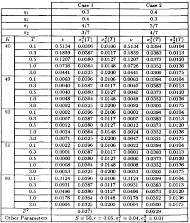
In Example 2.1 below, we perform some numerical experiment for the discrete-time model. However, as indicated in Remark 2.1, we do not intend to show the practical usefulness of this model, but ra,ther infer some intuitions behind.

Example 2.1. In this example, we assume that the underlying conditions have only two states, say good for state 1 and bad for state 2

(cf.

Figure 1). The current stock price 5 is fixed to be 50. We consider two cases where the transition probabilities of the underlying Markov chain

{Xn}

are given by III = 0.7 and

In

= 0.5 as Case 1, and III =

122

= 0.4 as Case 2. Note that

{Xn}

is ~tochastically monotone if and only if

III

+

In

?:

1. Hence, Case 1 assumes a stochasticallv monotone Markov chain while Case 2 does not. In Table 1, various values of Ci(n, 5, K): i = 1,2, AVG=L;=1 1r'iCi(n, 5, K) and CRR are listedlO

. It

is explicitly observed that Cl (Tt, 5, K) > C2 ( n, 5, K) in Case 1, as it should be, and even

in Case 2, although this case needs not be. Also, it is interesting to note that the CRR underprices all the cases with even the situation C2 ( n, 5, K) >CRR sometimes. [J

3 The Continuous-time Model

In this section, we derive an option pricing for the continuous-time model as a limit of (2.10). For this purpose, we let It be the length of each period and assume it sufficiently small. For the underlying process

{X,},

we set

J;j

=

%h

for i

1:-

j. The discrete-time Markov chain

{Xn}

then converges in distribution to a continuous-time Markov chain

{X(t),t

?:

O}, on the same state space S, governed by the infinitesimal generator Q = (qij) with q;; = -qi and qi = L#i %. Throughout this section, we assume that qi is bounded to eliminate inessential technical difficulties. Now, let Ili and ai denote the instantaneous mean rate

of return and the volatility of lhe stock price of the continuous-time model, respectively, when the underlying process is in state i. Then, assuming that the underlying process is independent of the stock price process (see footnote 6 for details), the exactly same

Markovian Volatility Option Pricing 157 P araIIleters r _ 1.05, u,

=

1 10 U2 - 1 07 d, - 0.80 d2

=

0 90 K n C,(n, S, K) C2(n,S,K) AVG CRR 40 2 13.8813 13.7544 13.8337 13.8252 3 15.6841 15.5292 15.6260 15.5749 4 17.2989 17.1986 17.2613 17.1810 5 18.8317 18.7586 18.8043 18.7916 6 20.3482 20.2679 20.3181 20.2759 CaseI 45 2 9.7254 9.4387 9.6179 9.3979 3 11.6402 11.3819 11.5434 11.5323 1rl = 4 13.5680 13.3131 13.4724 13.4088 11"2 = 5 15.2525 15.0615 15.1809 14.9865 6 16.8181 16.7064 16.7762 16.7348 50 2 6.4003 5.5093 6.0662 6.0138 3 8.1316 7.6840 7.9638 7.5932 4 9.9218 9.5783 9.7930 9.7686 5 11.9117 11.5752 11.7855 11.7158 6 13.6206 13.3653 13.5249 13.2921 55 2 3.1954 2.0765 2.7758 2.7697 3 5.3542 4.5176 5.0405 4.9801 4 6.9818 6.4764 6.7923 6.4223 5 8.6759 8.2909 8.5316 8.4745 6 10.6554 10.2658 10.5093 10.4322 60 2 0.2205 0.0000 0.1378 0.0000 3 2.7564 1.7287 2.3710 2.3669 4 4.6659 3.9176 4.3853 4.3174 5 6.1675 5.6873 5.9874 5.5920 6 7.8113 7.3985 7.6565 7.5722 K n C,(n,S,K) C2(n,S,K) AVG CRR 40 2 13.8421 13.7615 13.8119 13.7968 3 15.6150 15.5225 15.5803 15.5124 4 17.2543 17.1804 17.2266 17.1594 5 18.7861 18.7437 18.7702 18.7514 6 20.2902 20.2421 20.2722 20.2167 CaseZ 45 Z 9.6876 9.4784 9.6091 9.3622 3 11.5430 11.3739 11.4796 11.4521 11'"1 =

t

4 13.4440 13.2855 13.3845 13.2903 1r2 = ~ 5 15.1441 15.0106 15.0940 14.9360 6 16.7512 16.6751 16.7226 16.6590 50 2 6.1869 5.5879 5.9623 5.8216 3 8.0427 7.7004 7.9143 7.3918 4 9.7536 9.5455 9.6756 9.6216 5 11.7264 11.5085 11.6447 11.5339 6 13.4477 13.2787 13.3843 13.1012 55 2 2.9264 2.1748 2.6445 2.5367 3 5.0875 4.5102 4.8710 4.7203 4 6.8421 6.4480 6.6943 6.1690 5 8.4528 8.2314 8.3698 8.2542 6 10.4084 10.1481 10.3108 10.1864 60 2 0.1206 0.0000 0.0787 0.0000 3 2.4271 1.7189 2.1615 2.0578 4 4.3564 3.8425 4.1637 4.0109 5 5.9947 5.5981 5.8460 5.3115 6 7.5368 7.2975 7.4471 7.2800

158 M. Kijima & T. Yoshida

argument as in Cox, Ross and Rubinstein [7J shows that the stock price process converges in distribution to a stochastic process {S(

t), t

~

O}

satisfying the stochastic differential equation

dS(t)

S(t) = PX(tl dt

+

UX(tldW(t), (3.1 )

where {W(t),

t

~

O}

denotes the standard Brownian motion process independent of

{X(t)}.

For the bond price, we set p

=

erh in the discrete-time model. The bond price then converges to B(t)J B(O) = ert.

Let Ci(T, S, J<) be the price of a European call of the continuous-time model, where S

is the current stock price, T the time to maturity, K the exercise price and i the current state of the underlying process. Ci(T, S, K) can be obtained as a limit of (2.10). The proof of the next theorem is standard and is omitted. Note that the instantaneous mean rates Pi are irrelevant to option pricing.

Theorem 3.1. In the above continuous-time model, the option price satisfies the

fol-lowing set of partial differential equations:

(3.2)

Remark 3.1. If state i is absorbing so that %

=

0 for all j E S, then (3.2) for i E S

coincides with the partial differential equation obtained by Black and Scholes [2J. Also, since Ci(T, S, J<) is derived from (2.10) as a limit, the properties obtained in Section 2 hold under appropriate assumptions. For example, if the continuous-time Markov chain

{X(t)}

is stochastically monotone (see, e.g., Keilson [19]) and if 171

> ... >

Urn, then we

have C1(T, S, J<) ~ ... ~ Cm(T, S, J<). Since any diffusion process can be approximated

by a birth-death process (see footnote 5), which is necessarily stochastically monotone, the above result holds for any diffusion volatility model, provided that the state of volatility is appropriately ordered. 0

Another look at the solution of (3.2) is as follows. Let ti , i E S, denote the random total

time that

{X(t)}

is in state

i

during the time interval [0,

TJ.

Of course, L:~1 ti

=

T.

Given a realization of {X(t),O ~ t ~ T}, it is well known that the logarithm of the solution S(T) of (3.1) is distributed by the normal distribution having the variance u2_{(T)T, where}

(3.3)

and the option price is given by BS(u2_{(T)). Here, BS(x) denotes the option price obtained}

from the BS equation having volatility

y'x,

i.e.

10g(Sj J<)

+

rT

v'xT

~ =

v'xT

+

-2-' (3.4)

where <p(O

=

J~oo </>(u)du with </>(u)

=

-Jr;e-

u2

/2. Since {W(t)} and {X(t)} are independent

of each other, it follows that

Ci(T, S, K) = E[BS(u2(T))IX(0) = iJ, i E S,

(3.5)

which agrees with the expression obtained in Hull and White [15) and Scott [27J. Unfor-tunately, however, the probability distribution of u2_{(T) given X(O) = i is hard to obtain}

Markovian Volatility Option Pricing 159

except for m

=

2., i.e., the underlying process has 2 states. For m

=

2, it is known (see page

178

in Ross

[25])

that,

and, for s

<

T,

where

[3

denotes the beta distribution

n

(S)i( s)n-i

[3(sjT;k,n-k+1)=L~nCi

f

I -

_f

I=!;:

Hence, Ci(T, S,

K)

in (3.5) can be obtained from (3.6) through (3.8) as

C1(T, 8, J<) (3.6) (3.8) =

I

T + BS

(a~

+

a?

~

ai s) dPr[t1

~

sIX(O) = 1] (3.9)

BS(a2 ) _ S(a? - an

I

T- Pr[t1 ~ sIX(O) =

1]

1

2~

0

/a~T+(a;-ans

{

[log(Sj K)

+

rT

+

(a~T

+

(a? - a~)s)j2]21 d

x exp - 2(a~T

+

(a; _ ans)

J

s.

The last equality in (3.9) follows from integration by parts and since, by an algebra using (3.4), one has

BS'(x) =

SV;;

~(O

2yx (3.10)

(cf.

page 221 of Cox and Rubinstein [8]). Co(T, S, K) can be obtained similarly.

We next obtain some bounds for (3.5) that are useful in estimating the true value of the option price. For this purpose, the next lemma is the key. In what follows, we write

v(r, T, S,

f{)

=

~(F+

(log(Sj K)+ rT)2 - 1),

(3.11)

and assume 0'1 :> ...

>

am.

Lemma 3.1. The BS equation (3.4) is convex in x for x ~ v( r,

T, S,

K) and is concave otherwise.

Proof. From (3.10), one has

BS"(x) =

SVT

[~:~(O

+

_1_

d~ ~'(O]

.

4x.fi·

2ft

dx

Since ~'( u) = -u~( u) and since

d~ =

~

[_log(S/f{)

+

rT

+

VZt] ,

160 M. Kijima & T. Yoshida

it follows that

BSI/(x) = 5\1T

(-1

+

(log(5j f{)

+

rT)2 _ XT)

4>(~).

4xvlx xT 4

The lemma now follows at once. 0

Let 1"ij(T) = E[tjIX(O) =

il,

i.e., 1"ij(T) denotes the mean time that X(t) is in state j during the time interval [0, T] starting from X(O) = i, and let a}(T)

=

E[a2(T)IX(O)

=

i]. Then, from (3.3), one has

(3.12) Also, let

a?(T) -- a;

TJi =

_{ar -}

i E

S.

a;'

(3.13)

Note that "lid

+

(1-TJi)a;" = al(T). The next theorem provides an upper and lower bounds for (3.5).

Theorem 3.2. For any i E S, if a~::; v:= v(r,T,5,f{) then

BS(a;(T)) ::; C:;(T, S, K) ::; 'l/iBS(a;)

+

(1 - TJi)BS(a!), (3.14) whereas if a2

_>

_{v then}

m

-BS(a;(T)) :::: C;(T, 5, K) :::: TJiBS(a;)

+

(1 - TJ;)BS(a!), (3.15) where a;(T) and TJi are given in (3.12) and (3.13), respectively.

Proof. If a; ::; v, since the event a2_{(T) ::; a; is certain, BS(x) for this case is convex}

in x from Lemma 3.1. Hence, the first inequality in (3.14) holds by applying Jensen's inequality to (3.5). To prove the second inequality, let 1" be the random variable distributed as Pr[r = ail = TJi and Pr[1" = a~J= 1 - TJi. Then, since a! ::; a2

(T) ::; a; with probability one, we have a2_(T)

_--<c

_{r, where}

_--<c

_{denotes the stochastic convex ordering (see, e.g .. Stoyan}

[29]). The desired inequality follows, since BS(x) is convex in x for this case so that

E[BS(a2(T))IX{0)

=

i] ::;

E[BS(r)) = TJiBS(a;)

+

(1 - TJi)BS(a!).

(3.15) follows similarly. 0

Remark 3.2. It is easy to see that

(3.16)

where 8ij = 1 for i = j and 8iJ =: 0 otherwise. Taking the Laplace transform in (3.16) with

respect to T, one has

It follows that, in the matrix form,

Markovian Volatility Option Pricing 161

where,

1"j(S)

denotes the column vector whose components are TiiCs), ej the jth unit vector, I the identity matrix, and

Q

= (qij) the infinitesimal generator governing the Markov chain

{X(t)}. Tij(T) are then obtained by inverting: (3.17). For example, when m = 2,

(T) - q2 T

+

ql [1 -(ql+q2)T]

Tl1 - ql

+

q2 (ql

+

q2)2 - e , T12 (T) = T - Tl1 (T),

T22(T) and T21(T) are obtained by ql and q2 being replaced with q2 and ql, respectively, in the above equation. 0

Suppose that the continuous-time Markov chain {X(t)} is ergodic and let 1f' = (1f'j) be the stationary distribution of {X(t)}. Define 0-2 = 2::i!=1 7l"ja;' In the same spirit as for the discrete-time model, we want to compare 2::J~'1 7l"jCj(T, S, K) with BS(0-2). The next result follows from Jensen's inequality.

Theorem 3.3. If

ai ::; v

=

vCr,

T, S, K)

then m BS(0-2) ::; L :,rjCj(T, S, K), (3.18) j=1 whereas if a~ ~ v then m BS( 0-2) ~ L'f"iCj(T, 5, ](). (3.19) j=1

Proof. From the first inequality in (3.14), one has

m m

L7l"jBS(a;(T))~. L7l"jCj(T,S,K). (3.20)

j=1 j=1

But, since BS(J:) is convex in x if

ai ::;

v, the left hand side in (3.20) is greater than or equal to BS(2::J~1 7l"jaY(T)). On the other hand, since

(3.21) from (3.17) and since 1f'IQ = 0, premultiplying 1f'1 to (3.21) yields S21f'If"j(S) = 1f'j, where I

denotes the transpose. In the real domain, this means that 2::;:1 7l"iTij(T) = 7l"jT. 11. follows from (3.12) thal;

m

0-2

=

L 7l"ja;(T). (3.22) j=l

Therefore, (3.18) follows. The proof of (3.19) is similar. 0

Remark 3.3. It is well known (see, e.g., page 269 of <Jinlar [4]) that 7l"j

=

limT-+oe. Tij(T)/T

for any i E

S

so that, from (3.12),

Hence, 0-2 _{can be interpreted as the mean of the volatility during one unit of time in the}

long run. Also, it is known that

-2 l' 2() l' 1

~

2

a = lm a T = lm T ~ tjaj

T-+oo T-+oo j=1

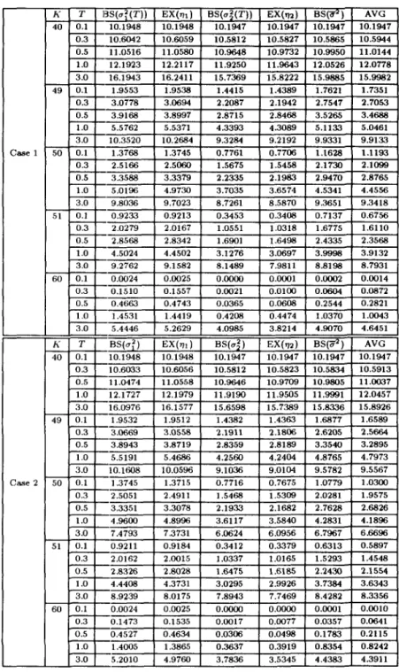
162 M. Kijima & T Yoshida CaseI Case 2 ql 0.3 0.4 q2 0.4 0.3 " I 4/7 3/7 "2 3/7 4/7

K T v at(T) ai(T) v at(T) a~(T)

40 0.1 0.5134 0.0396 0.0106 0.5134 0.0394 0.0104 0.3 0.1859 0.0387 0.0117 0.1859 0.0383 0.0113 0.5 0.1207 0.0380 0.0127 0.1207 0.0373 0.0120 1.0 0.0726 0.0364 0.0148 0.0726 0.0352 0.0136 3.0 0.0441 0.03205 0.0200 0.0441 0.0300 0.D175 49 0.1 0.0063 0.0396 0.0106 0.0063 0.0394 0.0104 0.3 0.0040 0.0387 0.0117 0.0040 0.0383 0.0113 0.5 0.0040 0.0380 0.0127 0.0040 0.0373 0.0120 1.0 0.0048 0.0364 0.0148 0.0048 0.0352 0.0136 3.0 0.0092 0.0325 0.0200 0.0092 0.0300 0.0175 SO 0.1 0.0002 0.0396 0.0106 0.0002 0.0394 0.0104 0.3 0.0007 0.0387 0.0117 0.0007 0.0383 0.0113 0.5 0.0012 0.0380 0.0127 0.0012 0.0373 0.0120 1.0 0.0024 0.0364 0.0148 0.0024 0.0352 0.0136 3.0 0.0071 0.0325 0.0200 0.0047 0.0321 0.0175 51 0.1 0.0022 0.0396 0.0106 0.0022 0.0394 0.0104 0.3 0.0001 0.0387 0.0117 0.0001 0.0383 0.0113 0.5 0.0000 0.0380 0.0127 0.0000 0.0373 0.0120 1.0 0.0008 0.0364 0.0148 0.0008 0.0352 0.0136 3.0 0.0053 0.0325 0.0200 0.0053 0.0300 0.D175 60 0.1 0.3124 0.0396 0.0106 0.3124 0.0394 0.0104 0.3 0.0931 0.0387 0.0117 0.0931 0.0383 0.0113 0.5 0.0496 0.0380 0.0127 0.0496 0.0373 0.0120 1.0 0.01 78 0.0364 0.0148 0.0178 0.0352 0.0136 3.0 0.0004 0.0325 0.0200 0.0004 0.0300 0.0175 if' 0.0271 0.0229 Other Parameters S

=

50. r

=

0.05, a

=

0.04, a~

=

0.01

Table 2: Parameter Values

with probability one, independent of the initial state. D

The content of Theorem 3.3 has an important implication. As explained in Section 2, (3.18) is a situation in which the BS equation underprices while it overprices if (3.19) holds. For deep out or in-the-money options with relatively short maturities, 10g(Sj J<) is big in the magnitude so that

v

=

v(r,T,

S, J<) in (3.11) is relatively large. Hence, it is likely that the BS equation underprices for such options. On the other hand, for near at-the-money options, 10g(S

j

J<) is negligible so that the 'V is, by Taylor's expansion, about r2T. This

value is very small for options with reasonable length of maturities and the BS equation is likely to overprice. Finally, we note that if

{X(t)}

is ergodic then, since (3.23) holds,

Cj(T, S, J<) converges to BS(O'2_{:1 with probability one as T -> 00.}

Example 3.1. In this example, we consider the continuous-time model with 2

under-lying states as in Example 2.1. The current stock price

S

is fixed to be 50 and we consider two cases where the transition intensities of the Markov chain

{X(t)}

are given by q12 = 0.3

and q21

=

0.4 as Case 1, and q12

=

0.4 and q21

=

0.3 as Case 2. Table 2 lists the parameter

values and 1t', v in (3.11), a-;(T) , i = 1,2, and 0'2. Note that, for near at-the-money options

(/{ =

49,50,51 in this example), v is smaller than a~

=

0.01 so that the condition for both (3.15) and (3.19) holds, and for the other values of J< the opposite condition holds except for T

2

1 of J< = 60. Also, it can be observed that a;(T) converge to 0'2 as T becomes large,

Markovian Volatih'ty Option Pricing 163

but the speed of convergence seems slow. Hence, the effect from the volatility's change over time can not be neglected for options with short length of maturities. This means that we should expect the current underlying state to a.ffect the price of such options considerably. In Table 3, various values of BS( anT)) and

EX(1Ji) = 1JiBS(O';) --(1 -1Ji)BS(O'i),

i

=

1,2, and BS(0'2) are listed. If v

2

O'r

=

0.04, BS(O'?(T)),

i

= 1,2, provide lower bounds for Ci = Ci(T, 5, K) while EX(1Ji) upper bounds. If v 5 O'i

=

0.01, on the other hand, the

BS(O't(T)) provide upper bounds while EX(1Ji) lower bounds. The bounds are surprisingly tight for near at-the-money options with relatively short maturities, say within a year. Also, we can see that the price C} is considerably hil~her than the price C2 for such options. For

long maturity options, we may need to calculate (3.9) directlyll. The last column termed AVG in Table 3 describes either upper or lower bounds of 1l'} C}

+

1l'2C2 according to whether

vSO'i

or

v

2 O'r, respectively. For example, when f{

=

50, AVG is calculated as

2

AVG =

L

1l';BS(0';(T)),

i=}

which, from (3.15), is greater than or equal to 1l'₁C} +1l'2C2' Therefore, from Table 3, one has 1l'_lC₁

+

1l'2C2 SBS(O'2), which in turn implies that the BS equation overprices for this case.

It can be explicitly observed that the BS equation overprices near at-the-money options whereas underprices deep out or in-the-money options with short maturities. Also, we can observe that C2 :; BS( 0'2) 5 C} in this example. Note that, in this example, only the case

T = 1.0 for ]{

=

60 satisfies neither v

2

O'i nor v 5 O'~. 0 4 Concluding Remarks

In this paper, we develop a Markovian volatility model, where the stochastic law of volatility is described in terms of a discrete state Markov chain. A discrete-time model is first constructed and it recursion formula for option pricing is derived. Based on the formula, we show that if the Markov chain is stochastically monotone then the higher current volatility the higher the option price. This result can be extended for any strong Markov process with continuous sample path (this includes difrusion processes), so that the result explains, to some extent, a well recognized phenomenon in actual option prices. This result is well known in practice but, to the authors' best knowledges, no theoretical explanation has been made in the literature. We then derive a continuous-time model as a limit of the discrete-time model where the stock price process follows a geometric Brownian motion process and the volatility dynamics follows a Markov chain on a discrete state space. If the stock price process is independent of the volatility (see footnote 6 for details), an option pricing formula is given as an integral of the BS equation. An explicit call valuation formula is given when the volatility takes one of two values, and some easily computable upper and lower hounds are obtained to estimate option prices based on the local convexity and concavity of the BS equation. The bounds are shown to be very tight especially for near at-the-money options with relatively short maturities, say within a year. Also, using the bounds, we succeed in explaining explicitly why the BS equation overprices near at-the-money options whereas it underprices deep out or in-the-money options.

Acknowledgment. The authors wish to thank the referees for their constructive com-ments which improve the original manuscript considerably. They also thank Hideki Iwaki for valuable discussions. One of the author (M K.) is supported in part by the fund endowed to the Research Association for Financial Engineering by the Toyo Trust and Banking Co. Ltd Mito Securities Co T.td amI the Dai-ichi Mutual Life Insurance Co.

llCalculation of (3.9) takes much time if (ql

+

q2)T is large. For, we need to take truncation point in (3.7) large so that the triple summation there becomes to matter.

164 M. Kijima & T. Yoshida

K T J3S(u2_{(T)) EX(!Jt} BS(u~(T)) EX(m) BS(52) AVG}

40 0.1 10.1948 10.1948 10.1947 10.1947 10.1947 10.1947 0.3 10.6042 10.6059 10.5812 10.5821 10.5865 10.5944 0.5 11.0516 11.0580 10.9648 10.9732 10.9950 11.0144 1.0 12.1923 12.2117 11.9250 11.9643 12.0526 12.0778 3.0 16.1943 16.2411 15.7369 15.8222 15.9885 15.9982 49 0.1 1.9553 1.9538 1.4415 1.4389 1.7621 1.7351 0.3 3.0778 3.0694 2.2087 2.1942 2.7547 2.7053 0.5 3.9168 3.8991 2.8115 2.8468 3.5265 3.4688 1.0 5.5162 5.5371 4.3393 4.3089 5.1133 5.0461 3.0 10.3520 10.2684 9.3284 9.2192 9.9331 9.9133 CaseI 50 0.1 1.3168 1.3745 0.7761 0.7706 1.1628 1.1193 0.3 2.5166 2.5060 1.5675 1.5458 2.1730 2.1099 0.5 3.3588 3.3319 2.2335 2.1983 2.9470 2.8165 1.0 5.0196 4.9730 3.7035 3.6514 4.5341 4.4556 3.0 9.8036 9.7023 8.7261 8.5870 9.3651 9.3418 51 0.1 0.9233 0.9213 0.3453 0.3408 0.1137 0.6156 0.3 2.0279 2.0167 1.0551 1.0318 1.6775 1.6110 0.5 2.8568 2.8342 1.6901 1.6498 2.4335 2.3568 1.0 4.5024 4.4502 3.1276 3.0697 3.9998 3.9132 3.0 9.2762 9.1582 8.1489 7.9811 8.8198 8.7931 60 0.1 0.0024 0.0025 0.0000 0.0001 0.0002 0.0014 0.3 0.1510 0.1557 0.0021 0.0100 0.0604 0.0812 0.5 0.4663 0.4743 0.0365 0.0608 0.2544 0.2821 1.0 1.4531 1.4419 0.4208 0.4474 1.0370 1.0043 3.0 5.4446 5.2629 4.0985 3.8214 4.9070 4.6451

K T BS(u2_{) EX('1J} BS(un EX('12) BS(,,2) AVG}

40 0.1 10.1948 10.1948 10.1947 10.1947 10.1947 10.1947 0.3 10.6033 10.6056 10.5812 10.5823 10.5834 10.5913 0.5 11.0474 11.0558 10.9646 10.9109 10.9805 11.0037 1.0 12.1727 12.1979 11.9190 11.9505 11.9991 12.0457 3.0 16.0976 16.1577 15.6598 15.7389 15.8336 15.8926 49 0.1 1.9532 1.9512 1.4382 1.4363 1.6877 1.6589 0.3 3.0669 3.0558 2.1911 2.1806 2.6205 2.5664 0.5 3.8943 3.8119 2.8359 2.8189 3.3540 3.2895 1.0 5.5191 5.4686 4.2560 4.2404 4.8765 4.7973 3.0 10.1608 10.0596 9.1036 9.0104 9.5782 9.5567 Case 2 50 0.1 1.3745 1.3115 0.7716 0.7675 1.0779 1.0300 0.3 2.5051 2.4911 1.5468 1.5309 2.0281 1.9575 0.5 3.3351 3.3078 2.1933 2.1682 2.7628 2.6826 1.0 4.9600 4.8996 3.6117 3.5840 4.2831 4.1896 3.0 7.4793 7.3731 6.0624 6.0956 6.7967 6.6696 51 0.1 0.9211 0.9184 0.3412 0.3379 0.6313 0.5897 0.3 2.0162 2.0015 1.0337 1.0165 1.5293 1.4548 0.5 2.8326 2.8028 1.6475 1.6185 2.2430 2.1554 1.0 4.4408 4.3731 3.0295 2.9926 3.7384 3.6343 3.0 8.9239 8.0175 7.8943 7.7469 8.4282 8.3356 60 0.1 0.0024 0.0025 0.0000 0.0000 0.0001 0.0010 0.3 0.1473 0.1535 0.0017 0.0077 0.0357 0.0641 0.5 0.4527 0.4634 0.0306 0.0498 0.1783 0.2115 1.0 1.4005 1.3865 0.3637 0.3919 0.8354 0.8242 3.0 5.2010 4.9760 3.7836 3.5345 4.4383 4.3911

Markovian Volatility Option Pricing 165

References

[1] Bailey, W. and Stulz, R. (1989). The pricing of stock index options in a general equi-librium model, Journal of Financial and Quantitative Analysis 24: 1-12.

[2] Black, F. and Scholes, M. (1973). The pricing of options and corporate liabilities, Journal of Political Economy 81: 637-659.

[3] Blackwell, D. (1955). On transient Markov process with a countable number of states and stationary transition probabilities, Annals of Mathematical Statistics 26: 654-658. [4] Cinlar, E. (HI_{75). Introduction to Stochasilc Processes, Prentice-Hall.}

[5] Cox, J.C., Ingersoll, J.E. and Ross, S.A. (1985). An intertemporal equilibrium model of asset prices, Econometrica 53:363-384.

[6] Cox, J.C., Ingersoll, J.E. and Ross, S.A. (1985). A theory of the term structure of interest rates, Econometrica 53:385-407.

[7] Cox, J.C., Ross, S. and Rubinstein, M. (19/'9). Option pricing: A simplified Approach, Journal of Fmancial Economics 7: 229-26:1.

[8] Cox, J.C. and Rubinstein, M. (1985). Option Markets, Prentice-Hall.

[9] Finnerty, J.K (1978). The Chicago boards options exchange and market efficiency, Journal of F1"nancial and Quantitative Analysis 13: 29-38.

[10] Follmer, H. and Schweizer, M. (1991). Hedging of contingent claims under incomplete information, Applied Stochastic Analysis, Davis, M.H.A. and Elliott, R.J. Ed., Gordon and Breach Science Publisher, 389-414.

[11] Harrison, M. and Kreps, D. (1979). Martingales and arbitrage in multiperiod securities markets, Journal of Economic Theory 20: 381-408.

[12] Harrison, M. and Pliska, S. (1981). Martingales and stochastic integrals in the theory of continuous trading, Stochastic Processe8 and their Applications 11: 215-260. [13] Heston, S.L. (1992). A closed form solution for options with stochastic volatility, with

application to bond and currency options, Yale University working paper.

[14] Hofmann, N., Platen, E. and Schweizer, M. (1992). Option Pricing Under Incomplete-ness and Stochastic Volatility, Mathematical Finance, 2/3: 153-187.

[15] Hull, J. and White, A. (1987). The pricing of options on assets with stochastic volatil-ities, The Journal of Finance 2: 281-300.

[16] Ingersoll, J.E. (1989). Theory of Financial Decision Making, Rowman and Littlefield. [17] Johnson, H.E. and Shanno, D. (1987). Option pricing when the variance is changing,

Journal of Financial and Quantitative Analysis 22: 143-151.

[18] Karlin, S. and Taylor, H.M. (1981). A Second Course in Stochastic Processes, Academic Press.

[19] Keilson, J. (1979). Markov Chain Models- Rarity and Exponentiality, Springer. [20] MacBeth, J. and Merville, L. (1979). An empirical examination of the Black-Scholes

call option pricing formula, Journal of Finance 34: 1173-1186.

[21] Madan, D.B. and Milne, F. (1991). Option pricing with V.G. martingale components, University of Maryland working paper.

[22] Madan, D.B. and Seneta, E. (1990). The variance Gamma (V.G.) model for share market returns, Journal of Business 63: .511-524.

[23] Merton, R. (1973). The theory ofrational option pricing, The Bell Journal of Economics and Management Science 4: 141-183.

[24] Naik, V. and Lee, M. (1990). General equilibrium pricing of options on the market portfolio with discontinuous return, The Review of Financial Studies 3: 493-521. [25] Ross, S.M. (1983). Stochastic Process, WiLey.

[26] Rubinstein, M. (1985). Nonparametric tests of alternative option pricing models using all reported trades and quotes on the 30 most active CBOE option classes from August 23, 1976 through August 31, 1978, Journal of Financial Economics 40: 455-480. [27] Scott, L.O. (1987). Option pricing when the variance changes randomly: theory,

166 M Kijima & T. Yoshida

(28) Stein, E.M. and Stein, J.C. (1991). Stock price distributions with stochastic volatility: An analytic approach, The Review of Financial Studies 4: 727-752.

(29) Stoyan, D. (1983). Comparison Methods for Queues and Other Stochastic Models, Wi-ley.

[30) Wiggins, J.B. (1987). Option values under stochastic volatility: Theory and empirical estimates, Journal of Financial Economics 19: 351-372.

Masaaki Kijima and Toshihiro Yoshida : Graduate School of Systems Management, The University of Tsukuba,