Searching a Hamiltonian Path in Giga-Node Graphs and Middle Levels Conjecture

全文

(1)Vol.2010-AL-130 No.9 2010/5/19 IPSJ SIG Technical Report 11111. Searching a Hamiltonian Path in Giga-Node Graphs and Middle Levels Conjecture. 11110. 11101. 11011. 10111. 01111. 11100. 11010. 11001. 10110. 10101. 10011. 01110. 01101. 01011. 00111. 11000. 10100. 10010. 10001. 01100. 01010. 01001. 00110. 00101. 00011. Manabu Shimada†1 and Kazuyuki Amano†1 The middle levels conjecture asserts that there is a Hamiltonian cycle in the middle two levels of 2k + 1-dimensional hypercube. The conjecture is known to be true for k ≤ 17 [I. Shields, B.J. Shields and C.D. Savage, Disc. Math., 309, 5271–5277 (2009)]. In this note, we verify that the conjecture is also true for k = 18 and 19 by constructing a Hamiltonian cycle in the middle two levels of 37- and 39-dimensional hypercube with the aid of the computer. We achieve this by introducing a new decomposition technique and an efficient algorithm for ordering the Narayana objects. In the largest case, our program could find a Hamiltonian path in a graph with ∼ 1.18 × 109 nodes in about 80 days on a standard PC.. M5 10000. 01000. 00100. 00010. 00001. 00000. Fig. 1 The hypercube Q5 and the middle levels graph M5 .. In this note, we verify that the conjecture is also true for k = 18 and 19 by constructing a Hamiltonian cycle in the middle two levels of 37- and 39-dimensional hypercube with the aid of the computer. We achieve this by plugging a new decomposition technique and an efficient algorithm for ordering the Narayana objects into a Hamiltonian path heuristic developed by Shields et al.4),5) . In the largest case, our program could find a Hamiltonian path in a graph with ∼ 1.18 · 109 vertices in about 80 days on a standard PC. The organization of this note is as follows. In Section 2, we briefly review the approach taken by Shields et al.4),5) for reducing the size of the problem. In Section 3, we describe an additional reduction that decomposes the problem into a number of smaller subproblems. In Section 4, we introduce an efficient algorithm for ordering the Narayana objects which was helpful for reducing the resource needed in the computation. Finally in Section 5, we summarize our computational results. Throughout the paper, n = 2k + 1 denotes the dimension of a hypercube.. 1. Introduction Let Qn denote the n-dimensional hypercube, i.e., Qn is a graph with 2n vertices, each vertex is labeled by an n-bit binary string and two vertices are adjacent iff their strings differ exactly in one bit. The i-th level of Qn is the set of vertices labeled by strings with exactly i ones. The middle levels graph is a subgraph of Q2k+1 induced by the middle two levels k and k + 1, and is denoted by M2k+1 (see Fig. 1). The middle levels conjecture asserts that the graph M2k+1 has a Hamiltonian cycle for every k. It appears as an “exercise” in Knuth’s book3) [Exercise 56, Sect. 7.2.1.3], in which the conjecture is credited to Buck and Wiedermann1) . In spite of considerable efforts, the conjecture remains open (see e.g., Johnson2) or Shields et al.4) and the references therein). It was shown to be true for k ≤ 11 by Moews and Reid, and for 12 ≤ k ≤ 15 by Shields and Savage5) and 16 ≤ k ≤ 17 by Shields et al.4) .. 2. Reducing the problem ( ) The Hamiltonicity of the middle levels graph, which has 2 nk vertices, can be reduced to the problem for finding a suitable Hamiltonian path in a smaller graph. †1 Dept. of Computer Science, Gunma University. 1. c 2010 Information Processing Society of Japan ⃝.

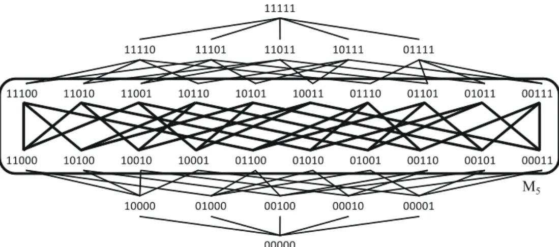
(2) Vol.2010-AL-130 No.9 2010/5/19 IPSJ SIG Technical Report σ. 1brun. 3brun. ρ(0001011). ρ(00011) group. ρ(00011). 2brun. 00011. 00110. 01100. 11000. 10001. 11100. 11001. 10011. 00111. 01110. ρ(0000111). ρ(0010011). ρ(0010101). reverse. ρ(0001101) σ. σ. σ. σ. R7 (k=3) 00101. ρ(00101). 01010. 10100. 01001. 10010. Fig. 3 The graph R7 and the decomposition of Rn based on “brun”. 11010. 10101. 01011. 10110. 01101. reverse. in Mn .. ρ(00101) group. R5. 3. Decomposition based on Runs. Fig. 2 The graph R5 and its relationship to the vertices of M5 .. Since the graph Rn is still huge (i.e., |R37 | ∼ 4.8 · 108 ), we divide Rn into a number of smaller graphs and search them individually and possibly in parallel. A run of a binary string x is a consecutive appearance of 1’s or 0’s in x. For example, we say that 000000 has one run and 001011 has four runs. We will divide Rn into three parts depending on the number of runs of strings in a vertex. Notice that ρ(x) may contain strings having different runs. We pick a string with k one’s such that it starts with 0 and ends with 1 as a representative of ρ(x), and the number of runs of this string is referred as the number of runs of ρ(x). Since this number is always even, we introduce a new unit called “brun” which is equal to two runs. Note that, in Rn , only ρ(0k+1 1k ) has 1 brun and only ρ(0(01)k ) has k bruns. In a preliminary experiment, we found that a decomposition based on the following three intervals is plausible (see Figs. 3 and 4). • Front part : 1 ∼ (⌊k/2⌋ − 1) brun(s) • Middle part : ⌊k/2⌋ ∼ (k − ⌊k/2⌋ + 1) bruns • Rear part : (k − ⌊k/2⌋ + 2) ∼ k bruns Note that, when k = 18, these three intervals are {1, 2, . . . , 8}, {9, 10} and {11, . . . , 18}. We will find a Hamiltonian path in each of these three graphs and then connect them to get a Hamiltonian path in Rn . In order to apply Lemma 1, we fix the start vertex of a path in the front part to ρ(0k+1 1k ) and the end vertex of a path in the rear part to ρ(0(01)k ). In addition, we should satisfy the additional. ( ) with nk /n vertices5) . For an n-bit binary sequence x = x1 x2 · · · xn , define the cyclic shift σ by σ(x) = x2 x3 · · · xn x1 . For every two vertices x and y in Mn , x and y are adjacent iff σ(x) and σ(y) are adjacent. This naturally introduces an equivalence relation ∼ on the set of vertices of Mn such that x ∼ y iff x = σ i (x) for some integer i. By noticing that that σ n (x) = x for every x, each equivalence class has n elements. A further reduction can be made by considering the complement. The complement of an n-bit binary string x = x1 x2 · · · xn is x ¯ = x¯1 x¯2 · · · x¯n . Note that two vertices x and y are adjacent iff x ¯ and y¯ are adjacent. By considering these two operations, the vertices of Mn is partitioned into |Mn |/2n classes, each of them has 2n vertices (Fig. 2). Here and hereafter, we denote the number of vertices of a graph G by |G|. For an n-bit binary sequence x, let ρ(x) denote this equivalence class including x, i.e., ρ(x) = {σ i (x), σ i (¯ x) | 0 ≤ i < n}. Let Rn denote the graph whose vertices are these equivalence classes and two vertices ρ(x) and ρ(y) in Rn are adjacent iff there is an edge between u and v in Mn for some u ∈ ρ(x) and v ∈ ρ(y). The following lemma, which was shown by Shields and Savage5) , guarantees that we can lift a Hamiltonian path in Rn to a Hamiltonian cycle in the middle levels graph. Lemma 1. If there is a Hamiltonian path in Rn starting from the vertex ρ(0k+1 1k ) and ending at the vertex ρ(0(01)k ), then there is a Hamiltonian cycle. 2. c 2010 Information Processing Society of Japan ⃝.

(3) Vol.2010-AL-130 No.9 2010/5/19 IPSJ SIG Technical Report. using a 32-bit integer par item. In this section, we give an efficient algorithm for ordering the vertices of our reduced graphs. A bit surprisingly, plugging this ordering scheme into a program gives a significant improvement of a running time of the program that will be shown in the next section. 4.1 View Vertices of Middle Levels as Catalan Objects The n-th Catalan number is the number of expressions containing n pairs of parentheses which are correctly matched and to be ) ( is well-known 1 2n C(n) = . n+1 n Notice that the number of vertices in Rn is equal to the k-th Catalan number C(k). This suggests that there is a bijection between the set of vertices of Rn and the set of correctly matched n pairs of parentheses. In the following, we identify a sequence of parentheses with a binary string under a mapping “(” ↔ “0” and “)” ↔ “1”. In addition, by a technical reason, we add one “0” to the top of the string. For example, we consider that “(()(()))” represents the string “000100111”. An 2k + 1 bit binary string starting with 0 is said to be correctly matched if it is corresponding to a correctly matched n pairs of parentheses. Fact 3. For every vertex ρ(x) in Rn , there is a unique correctly matched string in ρ(x).. requirements that (i) an end vertex of a path in the front part is adjacent to a start vertex of a path in the middle part, and (ii) an end vertex of a path in the middle part is adjacent to a start vertex of a path in the rear part. After some considerations, we pick strings hc(k, r) := 0k−r+1 (01)r 1k−r as terminals of paths. Note that ρ(hc(k, r)) has a maximum number of neighbors in vertices with r − 1 bruns and with r + 1 bruns, respectively. In addition, (i) hc(k, 1) = 0k+1 1k , (ii)hc(k, k) = 0(01)k , and (iii) for every i, ρ(hc(k, i)) and ρ(Rev(hc(k, i + 1))) are adjacent in Rn where Rev(x) denotes the reverse of a string x = x1 x2 · · · xn i.e., Rev(x) = xn · · · x2 x1 . We also use the following fact which can easily be verified. Fact 2. Let {ℓ, ℓ + 1, . . . , r} be a subset of {1, 2, . . . , k}. Suppose that there is a Hamiltonian path in an induced subgraph of Rn with vertices of at least ℓ bruns and at most r bruns that starts from ρ(x) and ends at ρ(y). Then there is a Hamiltonian path in the same graph that starts from ρ(Rev(x)) and ends at ρ(Rev(y)). For a Hamiltonian path P , let Rev(P ) denote a Hamiltonian path in a same graph whose existence is guaranteed by Fact 2. In summary, our search procedure is the following: First find a Hamiltonian path in each of three parts of the graph starting from ρ(hc(k, ℓ)) and ending at ρ(hc(k, r)) where ℓ and r are the left-end and right-end of each interval, and let denote these three paths as PF , PM and PR . Then connect PF , Rev(PM ) and PR in this order to get a Hamiltonian path in Rn which fulfills the condition in Lemma 1.. Proof. We should only consider a string with k one’s since no string with k + 1 one’s is correctly matched. Suppose that we represent a string by a path in the grid such that it goes upward when we read 0 and downward when we read 1. For example, a path for the string 0000111 is drawn as Fig. 5. It is clear that a string x is correctly matched iff the starting point of the path for x is located at the lowest level in the path and it is only the point on this level. Recall that ρ(x) contains every string that obtained from x by applying the cycle shift an arbitrary times. Note that, for every x with k one’s, a path for x ends at one step higher than the starting point of the path. Hence if we draw paths for x and σ i (x) for some i, a path for the substring that shifted backward in σ i (x) is drawn at one level higher than the original level (Fig. 6).. 4. Ordering of Vertices Each vertex of the graph Rn can naturally be stored using n bits of memory. However, this can be reduced by using an efficient ordering of the vertices. Indeed, since the number of vertices of Rn is less than 232 for n ≤ 39, we can store them Front part. k is even k is odd. 䊶䊶䊶䊶䊶䊶. Middle part. Rear part. 䊶䊶䊶䊶䊶䊶. Fig. 4 The decomposition of Rn . Each small circle represents an induced subgraph by the vertices with a specified brun.. 3. c 2010 Information Processing Society of Japan ⃝.

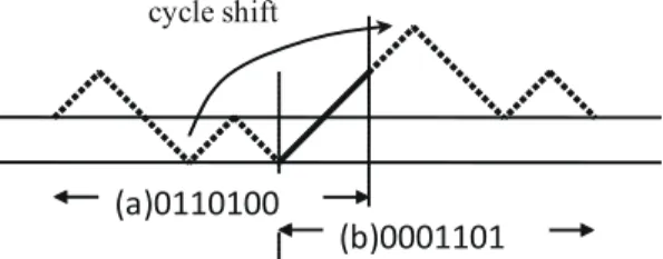
(4) Vol.2010-AL-130 No.9 2010/5/19 IPSJ SIG Technical Report. k p. Fig. 7 Cw (k, p) is equal to the number of left-right paths in the grid.. 0. 0. 0. 0. 1. 1. 1 graphically smaller than x. Hence if we can count the number of strings smaller than x ˜ for a given prefix x ˜, then the ordering of x can easily be computed. For example, the ordering of the string 0010101 in a set S ⊆ {0, 1}7 can be computed as the sum of the numbers of strings in S starting from 000, 00100 and 0010100. Let Pℓ ⊆ {0, 1}2ℓ+1 be the set of correctly matched strings of length 2ℓ + 1. For a prefix x ˜ ∈ {0, 1}t with t ≤ 2ℓ + 1, the number of strings in Pℓ starting with x ˜ is shown to be ( ) p+1 2k − p Cw (k, p) = , (1) k+1 k−p. Fig. 5 A path for the string “0000111”.. cycle shift. (a)0110100 (b)0001101 σ 5 (x). Fig. 6 A path for x = 0110100 (a) and for = 0001101 (b). A dotted line represents a path for the substring ‘01101’ which goes backward by the cycle shift in (b).. where p = ♯0 (˜ x) − ♯1 (˜ x) − 1 and k = ℓ − ♯1 (˜ x). Here we denote the number of 0’s and 1’s in x ˜ by ♯0 (˜ x) and ♯1 (˜ x), respectively. Intuitively, p denotes the height of the end point of a path for x ˜ and k denotes the number of “remaining” one’s in a string (see Fig. 7). Note that these numbers are known as the Catalan Triangle (see e.g., the sequence A009766 of7) ). Using Eq. (1), we can calculate the lexicographical ordering of a vertex ρ(x) efficiently. For example, the ordering of ρ(0010101) is given by Cw (3, 2) + Cw (2, 2) + Cw (1, 2) = 3 + 1 + 0 = 4. 4.3 Runs and Narayana Numbers Since we decompose the graph Rn into smaller parts, it is desirable to give an efficient ordering algorithm for the set of vertices of these decomposed graphs. By a similar argument to that in Section 4.1, the number of vertices of Rn with r bruns is shown to be ( )( ) 1 k k N (k, r) = , k r r−1 which is known as the Narayana numbers. N (k, r) is the number of correctly matched k pairs of parentheses that contains the subsequence “()” exactly r times. Note that the Catalan numbers are represented by the sum of the Narayana. By this observation, it is easy to see that a correctly matched string in ρ(x) can be obtained by (i) draw a path for x, and pick the rightmost point among all points on the lowest level of the path, and (ii) shift x so that this point becomes the top of the resulting string. It is also easy to see that every other string in ρ(x) is not correctly matched. This guarantees the uniqueness and hence completes the proof. By this fact, there is a bijection from the set of vertices in Rn to the Catalan objects, i.e., the vertices in Rn are uniquely mapped to integers {0, 1, . . . , C(k) − 1}. 4.2 Lexicographical Ordering for Catalan Objects In our programs, we number vertices ρ(x) in Rn according to the lexicographical ordering (starting from 0) of a correctly matched string in ρ(x). Obviously, the ordering of a string x is equal to the number of strings lexico-. 4. c 2010 Information Processing Society of Japan ⃝.

(5) Vol.2010-AL-130 No.9 2010/5/19 IPSJ SIG Technical Report. numbers, i.e., C(k) =. k ∑. 3 and the ordering described in Section 4.3 are included. N (k, i).. Table 1 Running time to find a Hamiltonian cycle in the middle levels graph. i=1. k. It is also shown that the lexicographical ordering of a string x in the set of correctly matched strings with r bruns can be efficiently computed using the following formula: ( )( ) k + (p − 1)(r − 1) k−p k Nw (k, p, r) = , k(k − p − r + 1) r r−1 that represents the number of correctly matched strings of which the meanings of p and k are the same as in Eq. (1) and r denotes the ‘remaining’ number of the subsequence “()”. A detailed discussion on how to compute the ordering for such Narayana objects will be appeared in the full version of this note.. Base. w/Decomp.. w/Ordering Front. 8 9 10 11 12 13 14 15 16 17 18 19. 5. Computational Results We develop a program for finding a Hamiltonian path for decomposed graphs based on the algorithm proposed by Shields et al.5) in which we represent the vertices of graphs by the ordering described in Section 4. Using this program, we have succeeded to find a desired Hamiltonian path for every three parts, i.e., the front, middle, rear parts of Rn for every 8 ≤ k ≤ 19, which shows the Hamiltonicity of the middle levels graphs for k ≤ 19. Note that, for smaller values of k, our decomposition schema would not work. The computational results are summarized in Table 1. Our program is executed on a PC with an Intel Xeon processor of 2.26 GHz and 24 GB of memory available. Note that the maximum memory used in our experiments was about 23 GB. We show the elapsed time in seconds, and the case that takes less than 1 second is shown as 0. The second column shows the elapsed time of a base program to find a path in the entire graph Rn . In a base program, we don’t use our ordering scheme and vertices are stored as n-bit strings. The third column shows the longest elapsed time of a base program for finding a path in each of three decomposed graphs. The fourth column shows the elapsed time of a program with the ordering technique for the entire graph Rn . The later columns show the elapsed time of a program in which both techniques, i.e., the decomposition described in Section. 0 0 0 1 7 51 542 7,657 88,795 -. 0 0 0 1 5 45 290 3,003 29,948 542,821 -. 0 0 0 1 6 30 182 1,984 17,130 195,330 -. 0 0 0 0 2 2 40 133 3,143 15,226 627,204 ∼4.85M (56.1days). w/Decomp.+Ordering Middle Rear 0 0 0 1 4 22 71 477 2,762 25,329 511,342 ∼ 7.01M (81.1days). 0 0 0 0 1 3 26 83 1,785 6,410 359,015 ∼ 2.33M (26.9days). Max 0 0 0 1 4 22 71 477 3,143 25,329 627,204 ∼ 7.01M (81.1days). A bit surprisingly, introducing the ordering into a search program gives a significant improvement of the running time. The combination of our two techniques reduces the running time by a factor of about 30 when k = 16. For k = 19, the number of vertices of the front, middle and rear parts of the graph is 291, 580, 993, 1, 184, 101, 205 and 291, 580, 993, respectively. Notice that the running time (per one vertex) is the longest for the front part of the graph. This suggests that finding a Hamiltonian path is harder for a graph consisting of vertices with smaller number of runs than that with larger number of runs. The source codes of the programs we used as well as some additional data are available on the web page6) . References 1) M.Buck and D.Wiedermann, Gray Codes with Restricted Density, Disc. Math., 48, 163–171 (1984) 2) J.R. Johnson, Long Cycles in the Middle Two Layers of the Discrete Cube, J.Combin. Theory Ser. A 105 (2), 255–271 (2004) 3) D.E.Knuth, The Art of Computer Programming Volume 4, Fascicle 3, AddisonWesley Pub (2005) 4) I.Shields and B.J.Shields and C.D.Savage, An Update on the Middle Levels Prob-. 5. c 2010 Information Processing Society of Japan ⃝.

(6) Vol.2010-AL-130 No.9 2010/5/19 IPSJ SIG Technical Report. lem, Disc. Math., 309, 5271–5277 (2009) 5) I. Shields and C.D. Savage, A Hamilton Path Heuristic with Applications to the Middle Two Levels Problem, Congressus Numerantium, 140, 161-178 (1999) 6) M.Shimada and K.Amano, Supplement of the paper available at http://www.cs.gunma-u.ac.jp/~amano/mlc/index.html 7) N.J.A.Sloane, The On-Line Encyclopedia of Integer Sequences, http://www2.research.att.com/~njas/sequences/. 6. c 2010 Information Processing Society of Japan ⃝.

(7)