Intersection dimension of bipartite graphs

全文

(1)Vol.2014-AL-148 No.4 2014/6/13. IPSJ SIG Technical Report. Intersection dimension of bipartite graphs Steven Chaplick1,a). Pavol Hell2,b) Yota Otachi3,c) Ryuhei Uehara3,e). Toshiki Saitoh4,d). Abstract: We introduce a concept of intersection dimension of a graph with respect to a graph class. This generalizes Ferrers dimension, boxicity, and poset dimension, and leads to interesting new problems. We focus in particular on bipartite graph classes defined as intersection graphs of two kinds of geometric objects. We relate well-known graph classes such as interval bigraphs, two-directional orthogonal ray graphs, chain graphs, and (unit) grid intersection graphs with respect to these dimensions. As an application of these graph-theoretic results, we show that the recognition problems for certain graph classes belong to NP. Keywords: Ferrers dimension, Boxicity, Unit grid intersection graph, Segment-ray graph. 1.. Introduction. Given a family F of sets, the intersection graph of F is the graph in which each set in F is a vertex, and two vertices are adjacent if and only if the corresponding sets intersect. A typical example, when F is a family of intervals on a line, yields the well-known class of interval graphs. Interval graphs have linear-time recognition algorithms [2], [9], and nice forbidden structure characterizations. (For instance, the theorem of Lekkerkerker and Boland [21] characterizes interval graphs by the absence of induced cycles of length four and five, and the absence of asteroidal triples.) It is natural to study a bipartite version of intersection graphs: given two families F and F ′ of sets, the intersection bigraph of F, F ′ is the bipartite graph in which each set in F is a red vertex, each set in F ′ is a blue vertex, and a red vertex is adjacent to a blue vertex if and only if the corresponding sets intersect. When both F and F ′ are families of intervals on a line, we obtain interval bigraphs studied in [22], [27]. We denote the class of interval bigraphs by IBG. While the recognition of interval bigraphs is polynomial (in time O(n5 m6 log n) [22]), there is no efficient algorithm known, and no characterization in terms of forbidden substructures. It turns out that there are bet1. 2. 3. 4. a) b) c) d) e). Institut f¨ ur Mathematik, Technische Universit¨ at Berlin, Berlin, Germany. School of Computing Science, Simon Fraser University, Burnaby, B.C., Canada V5A 1S6. School of Information Science, Japan Advanced Institute of Science and Technology. Asahidai 1-1, Nomi, Ishikawa 923-1292, Japan Graduate School of Engineering, Kobe University, Rokkodai 1-1, Nada, Kobe, 657-8501, Japan. [email protected] [email protected] [email protected] [email protected] [email protected]. ⓒ 2014 Information Processing Society of Japan. ter bipartite analogues of interval graphs. A two-directional orthogonal ray graph, or 2DOR graph, is an intersection bigraph of a family F of upward rays, and a family F ′ of rightward rays, in the plane [29]. These graphs were introduced in connection with defect tolerance schemes for nano-programmable logic arrays [25], [33]. There are several reasons these 2DOR graphs might be considered better bipartite analogues of interval graphs, including an ordering characterization [18], [29], and a Lekkerkerker-Boland type characterization [10], both analogous to the characterizations for interval graphs. Moreover, it follows from [10] that the class 2DOR plays the same role for bigraphs as the class of interval graphs play for graphs, as far as polynomial solvability of certain constraint satisfaction problems is concerned. Other equivalent definitions, and forbidden structure characterizations of the class 2DOR can be found in [10], [16], [17]. Several other graph classes can be defined as intersection bigraphs of two families F, F ′ . When both F and F ′ are inclusion-free families of intervals on a line, we obtain the class of proper interval bigraphs which turns out to be the same as the better known class BPG of bipartite permutation graphs [17], see below. When F is a family of points, and F ′ a family of rightward rays, in a line, we obtain the class CHAIN of chain graphs (cf. below). When F is a family of vertical segments, and F ′ a family of horizontal segments, in the plane, we obtain the class GIG of grid intersection graphs. Several other examples are included in the paper. We note that the following inclusions are well known or easy to derive CHAIN ⊆ BPG ⊆ IBG ⊆ 2DOR ⊆ GIG. We now introduce our concept of intersection dimension. Let G = (V, E) and G′ = (V ′ , E ′ ) be two graphs. The intersection G∩G′ of G and G′ is the graph (V ∩V ′ , E ∩E ′ ). For 1.

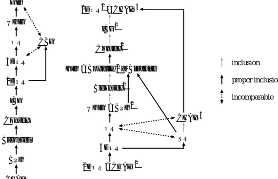
(2) IPSJ SIG Technical Report. two graph classes C and C ′ , we define the pairwise intersec× C ′ = {G ∩ G′ : G ∈ C, G′ ∈ C ′ }. We tion of C and C ′ as C ∩ k also write C = {G1 ∩ G2 ∩ · · · ∩ Gk : Gi ∈ C for 1 ≤ i ≤ k}. If both C and C ′ are closed under taking induced subgraphs, × C ′ = {G ∩ G′ : G ∈ C, G′ ∈ it is easy to check that C ∩ C ′ , V (G) = V (G′ )}. Since every graph class in this paper is closed under taking induced subgraphs, we shall from now on use the latter equality, and assume that the vertex sets of the two graphs are the same, when defining the pairwise intersection of graph classes. The dimension of a graph G with respect to the graph class C is the minimum k such that G ∈ C k . In the discussion below we shall point out how this definition generalizes Ferrers dimension, boxicity, cubicity, and poset dimension. We are particularly interested in expressing one graph class as a (subset of a) power of another graph class. It turns out that there are several natural statements of this kind. See the following section for a summary of results. 1.1 Our results Among other results we will show that 2DOR = CHAIN2 , GIG ⊆ CHAIN4 , and UGIG = BPG2 . We will also show that several of these inclusions are proper. See Fig. 1 for the summary of our results. The characterizations we will present give compact representations for several graph classes, which implies that the recognition problems for those graph classes belong to NP. Combining with a recent result of Mustat¸ˇa and Pergel [23], we will conclude that the problems are NP-complete. We also consider forbidden matrix characterizations of graph classes. It is known that some important classes of graphs such as CHAIN, 2DOR, and GIG have characterizations in terms of forbidden submatrices of their biadjacency matrix. We will show that a 2 × 3 forbidden matrix characterizes the class of intersection bigraphs of horizontal segments and upward rays. Finally, we will show that two well-known concepts of graph dimension, boxicity and Ferrers dimension, are essentially the same for bipartite graphs.. 2.. Preliminaries. A graph G = (V, E) is a bipartite graph (or a bigraph for short) with bipartition (X, Y ) if V is partitioned into X and Y in such a way that each edge of G has one endpoint in X and the other in Y . We denote such a bigraph by (X, Y ; E). A biadjacency matrix MB of a bigraph B = (X, Y ; E) is a 0-1 matrix with the rows indexed by the vertices of X and the columns indexed by the vertices of Y such that {x, y} ∈ E if and only if the corresponding entry of MB is 1. For m × n 0-1 matrices M ′ and M ′′ , their intersection M = M ′ ∩ M ′′ is the 0-1 matrix such that Mi,j = 1 if and ′ ′′ only if Mi,j = Mi,j = 1. The neighborhood of a vertex v in a graph G, denoted NG (v), is the vertices adjacent to v in G.. ⓒ 2014 Information Processing Society of Japan. Vol.2014-AL-148 No.4 2014/6/13. 2.1 Graph classes Here we define the graph classes we deal with in this paper. We also introduce some important properties of them. For their inclusion relations and other known results for them, the readers can refer to the standard textbooks in this field [3], [12], [32]. For a graph class C, the recognition problem of C is the problem deciding whether a given graph belongs to C. 2.1.1 Chain graphs and Ferrers diagrams A bipartite graph B = (X, Y ; E) is a chain graph if there is an ordering (x1 , x2 , . . . , xp ) on X such that NB (x1 ) ⊇ NB (x2 ) ⊇ · · · ⊇ NB (xp ). It is easy to see that if there exists such an ordering on X, then there exists an ordering (y1 , y2 , . . . , yq ) on Y such that NB (y1 ) ⊇ NB (y2 ) ⊇ · · · ⊇ NB (yq ). Chain graphs are also known as difference graphs and Ferrers bigraphs. It is known that chain graphs are exactly 2K2 -free bigraphs [13]. The class of chain graphs is denoted by CHAIN. A 0-1 matrix has the Ferrers property if its rows and columns can be reordered so that 1’s in each row and column appear consecutively with the rows left-justified and the columns top-justified. The reordered matrix is called a Ferrers diagram. It is easy to see that a matrix has the Ferrers property if and only if it has none of the following 2 × 2 matrices as a submatrix: ( ) ( ) 0 1 1 0 , . (1) 1 0 0 1 Since chain graphs are exactly the 2K2 -free bigraphs, it is easy to see that chain graphs are exactly the bigraphs whose biadjacency matrices have the Ferrers property. 2.1.2 Bipartite permutation graphs, convex graphs, biconvex graphs, interval bigraphs, and chordal bipartite graphs A graph G = (V, E) with V = {1, 2, . . . , n} is a permutation graph if there is a permutation π over V such that {i, j} ∈ E(G) if and only if (i − j)(π(i) − π(j)) < 0. A graph is a bipartite permutation graph if it is bipartite and a permutation graph. The class of bipartite permutation graphs is denoted by BPG. Several equivalent definitions of the class BPG are collected in [17]. An ordering < of X in a bipartite graph B = (X, Y ; E) has the adjacency property if for every vertex y in Y , N (y) consists of vertices that are consecutive in the ordering < of X. A bipartite graph (X, Y ; E) is convex if there is an ordering of X or Y that fulfills the adjacency property. A bipartite graph (X, Y ; E) is biconvex if there are orderings of X and Y that fulfill the adjacency property. We denote the classes of convex bipartite graphs and biconvex bipartite graphs by Convex and Biconvex, respectively. A bi-interval representation of a bigraph B = (U, V ; E) is a pair (IU , IV ) of sets of closed intervals such that IU = {Iu = [ℓu , ru ] : u ∈ U } and IV = {Iv = [ℓv , rv ] : v ∈ V }, and {u, v} ∈ E for u ∈ U and v ∈ V if and only if Iu ∩ Iv ̸= ∅. A bi-interval representation (IU , IV ) is unit if for each interval [ℓ, r] ∈ IU ∪ IV , r − ℓ = 1. 2.

(3) Vol.2014-AL-148 No.4 2014/6/13. IPSJ SIG Technical Report. GIG. 2DOR2 = CHAIN4. UGIG OR. IBG2 CBG. Convex2. 3DOR. inclusion. GIG = Boxicity 2 ∩ Bipartite 2DOR. proper inclusion. Biconvex2. incomparable. IBG. UGIG = BPG2. Convex. CHAIN3. OR SR. Biconvex 3DOR BPG. 2DOR = CHAIN2. CHAIN Fig. 1. (Left) Known hierarchy. (Right) New hierarchy based on intersection dimension.. A bigraph is a chordal bipartite graph if every induced cycle is of length four. The class of chordal bipartite graphs is denoted by CBG. 2.1.3 Orthogonal ray graphs A bipartite graph B = (X, Y ; E) is an orthogonal ray graph if there is a pair (RX , RY ) of families of rays (or half-lines) such that RX = {Rx : x ∈ X} is a family of pairwise non-intersecting horizontal rays, RY = {Ry : y ∈ Y } is a family of pairwise non-intersecting vertical rays, and {x, y} ∈ E if and only if Rx and Ry intersect. We call such a pair (RX , RY ) an orthogonal ray representation of B. We denote the class of orthogonal ray graphs by OR. Note that in a representation of an orthogonal ray graph horizontal rays can go rightward and leftward and vertical rays can go upward and downward. If we restrict horizontal rays to be only rightwards, then we have 3-directional orthogonal ray graphs. Furthermore, if we restrict horizontal rays to be only rightwards and vertical rays to be only upwards, then we have 2-directional orthogonal ray graphs. We denote the classes of 3-directional orthogonal ray graphs and 2-directional orthogonal ray graphs by 3DOR and 2DOR, respectively. For the class 2DOR, several nice characterizations are known (see e.g. [10], [16], [18], [26], [27], [28], [29]). Among those characterizations, the followings are useful for our purpose. In this language they appear in [28], [29], in an equivalent graph theoretic form they are given in [16], [18]. Theorem 2.1. For a bigraph B, the following conditions are equivalent: ( 1 ) B is a 2-directional orthogonal ray graph; ( 2 ) B is γ-freeable; that is, the rows and columns of a biadjacency matrix of B can be independently permuted so that no 0 has a 1 both below it and to its right;. ⓒ 2014 Information Processing Society of Japan. ( 3 ) B is of Ferrers dimension at most 2. (The Ferrers dimension of a bigraph is defined in Section 2.1.8.) There are other equivalent characterizations of the class 2DOR, as suggested in the introduction. In particular, 2DOR is precisely the class of bigraphs whose complements are circular arc graphs [29]; because of the characterizations of the latter class in [10], [16], [17], one obtains several other forbidden structure characterizations of 2DOR, in terms of the absence of induced cycles and bipartite versions of asteroids, in terms of the so-called invertible pairs, and in other terms. It is known that the recognition of 2DOR can be done in polynomial time [10], [29], while it is open for 3DOR and OR. Recently, Felsner, Mertzios, and Mustat¸ˇ a [11] have shown that if the direction (right, left, up, or down) for each vertex is given, then it can be decided in polynomial time whether a given graph has an orthogonal ray representation in which each vertex has the given direction. 2.1.4 Grid intersection graphs A bipartite graph B = (X, Y ; E) is a grid intersection graph if there is a pair (SX , SY ) of families of segments such that SX = {Sx : x ∈ X} is a family of pairwise nonintersecting horizontal segments, SY = {Sy : y ∈ Y } is a family of pairwise non-intersecting vertical segments, and {x, y} ∈ E if and only if Sx and Sy intersect. We call such a pair (SX , SY ) a grid intersection representation of B. A bipartite graph is a unit grid intersection graph if it has a grid intersection representation in which each segment if of length 1. We denote the classes of grid intersection graphs and unit grid intersection graphs by GIG and UGIG, respectively.. 3.

(4) Vol.2014-AL-148 No.4 2014/6/13. IPSJ SIG Technical Report. 2.1.5. Recognition problems and inclusion relations For the graph classes introduced above, the following relations are known [3], [24], [29]: CHAIN ⊊ BPG ⊊ Biconvex ⊊ Convex ⊊ IBG ⊊ 2DOR ⊊ 3DOR ⊊ OR ⊊ UGIG ⊊ GIG. Also it is known that 2DOR ⊊ CBG [29], and that CBG is incomparable to 3DOR and GIG [24]. It is known that the recognition problems of CHAIN [15], BPG [30], Biconvex [32], Convex [32], IBG [22], 2DOR [29], and CBG [31] can be solved in polynomial time. On the other hand, it is known that the recognition problems of GIG [20] and UGIG [23], [34] are NP-complete. The complexity of the recognition problems of 3DOR, OR, and SR is not known. Note that even if three graph classes A, B, and C satisfy A ⊆ B ⊆ C and the recognition problems of A and C are both polynomial-time solvable (NP-hard), it does not mean the recognition problem of B is polynomial-time solvable (NP-hard, resp.). 2.1.6 Other graphs The d-dimensional hypercube Hd is the graph with 2d vertices in which the vertices corresponds to the subsets of {1, . . . , d} and two vertices are adjacent if and only if the symmetric difference of the corresponding sets is of size 1. Let Ka,b denote the complete bipartite graph having a vertices in one side and b vertices in the other side. We denote by Kn,n − nK2 the graph obtained by removing a perfect matching from the complete bipartite graph Kn,n . 2.1.7 Boxicity and cubicity An interval graph is the intersection graph of closed intervals on the real line. A unit interval graph is the intersection graph of closed unit intervals on the real line. We denote the classes of interval graphs and unit interval graphs by INT and UINT, respectively. The boxicity of a graph G is the minimum integer k such that G ∈ INTk , and the cubicity of G is the minimum integer k such that G ∈ UINTk . It is known that given a graph, deciding whether its boxicity (or cubicity) is at most 2 is NP-complete [4], [20]. 2.1.8 Ferrers dimension The Ferrers dimension fd(B) of a bigraph B is the smallest number of Ferrers bigraphs whose intersection is B. That is, fd(B) is the minimum integer k such that B ∈ CHAINk . As we will see in Section 3, if B = (X, Y ; E) and fd(B) = k, then there are Ferrers bigraphs Bi = (X, Y ; Ei ) for 1 ≤ i ≤ ∩ k such that B = 1≤i≤k Bi . That is, we can assume all the graphs B and Bi , 1 ≤ i ≤ k, have the same bipartition. A Ferrers digraph D = (V, A) is a digraph whose adjacency matrix has the Ferrers property. The Ferrers dimension fd(D) of a digraph D is the smallest number of Ferrers digraphs whose intersection is D. 2.1.9 Poset dimension The poset dimension pd(P ) of a poset P is the minimum integer k such that there exist k linear extensions of P such ⓒ 2014 Information Processing Society of Japan. that for any two elements x, y of P , x < y in P if and only if x < y in all the linear extensions. The Ferrers dimension fd(P ) of a poset P is the Ferrers dimension of the digraph defined in such way that the vertices are the elements of P and there is an arc (u, v) if and only if u < v. Cogis [8] showed that for any poset P , fd(P ) = pd(P ). A poset is of height 2 if every element is either a minimal element or a maximal element. The underlying graph of a height-2 poset is the bigraph B = (X, Y ; E) such that X is the set of minimal elements, Y is the set of maximal elements, and {x, y} ∈ E if and only if x < y. It is easy to see that any bigraph is the underlying graph of some poset of height 2.. 3.. Bigraph intersection dimension. For two bipartite graph classes, if one of them is closed under disjoint union and taking induced subgraphs, we may assume that the bipartitions of G and G′ are the same when taking their intersection. More precisely, we have the following lemma. Lemma 3.1. Let B and B′ be bipartite graph classes. If at least one of them is closed under disjoint union and taking × B ′ = {(X, Y ; E) ∩ (X, Y ; E ′ ) : induced subgraphs, then B ∩ ′ (X, Y ; E) ∈ B, (X, Y ; E ) ∈ B′ }. Unfortunately, CHAIN is not closed under disjoint union. For example, K2 is a chain graph but 2K2 is not. It is the only exception in this paper. Fortunately, we have the following lemma for chain graphs. Lemma 3.2. CHAIN2 = {(X, Y ; E) ∩ (X, Y ; E ′ ) : (X, Y ; E), (X, Y ; E ′ ) ∈ CHAIN}.. X1 ∩ X2. Y1 ∩ Y2. X1 ∩ Y2. X1 ∩ X2. Y1 ∩ X2. Y1 ∩ Y2. H1′ Fig. 2. X1 ∩ Y2. Y1 ∩ X2 H2′. Intersection of two chain graphs.. By Lemmas 3.1 and 3.2, we can assume that the bipartitions of two graphs are the same when we are defining the pairwise intersection of two graph classes, since, in this paper, either one of them is closed under disjoint union or both of them are the class of chain graphs.. 4.. (P, Q; D)-Bigraphs. We introduce the notion of (P, Q; D)-bigraphs, where a bigraph B = (U, V, E) is said to be an (P, Q; D)-bigraph if and only if for some domain D (e.g., the real number line R) each vertex in u ∈ U can be represented as a type P subset Pu of D and each vertex v ∈ V can be represented as a type Q subset Qv of D such that for every u ∈ U, v ∈ V, {u, v} ∈ E if and only if Pu ∩ Qv ̸= ∅. For example, in this setting, interval bigraphs are (interval, interval, R)-bigraphs. We will use (P, Q; D) to denote the class of (P, Q; D)-bigraphs. 4.

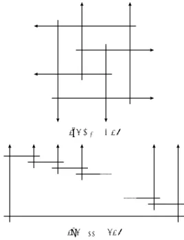
(5) Vol.2014-AL-148 No.4 2014/6/13. IPSJ SIG Technical Report. Our discussion will focus on the cases when P, Q are the following subsets of R: points, rays, unit-intervals, and intervals; and the following axis-aligned subsets of R2 : points, rays, unit-segments, segments, squares, and rectangles. Note that, for rays, we will use →, ↓, ←, and ↑ to denote the rightward, downward, leftward, and upward rays respectively. Moreover, when we refer to a ray r (rather than using a specific arrow), r can be any axis-aligned ray from the domain.. borhoods are pairwise incomparable. This is formalized in the following proposition. Proposition 4.5. If a bigraph B = (X, Y ; E) is (ray, point; R) where each x ∈ X is a ray then for every {x, x′ , x′′ } ⊆ X and every y ∈ Y , there exists x∗ ∈ {x, x′ , x′′ } and x∗∗ ∈ {x, x′ , x′′ } \ {x∗ } such that N (x∗ ) ⊆ N (x∗∗ ) or N (x) ⊆ N (x′′ ).. a. b. c. a. b. 4.1 (P, Q; R)-Bigraphs We begin with some easy observations characterizing CHAIN, Convex, and Biconvex bigraphs as (P, Q; D)bigraphs (see Proposition 4.1). This is followed by a couple essential lemmas that we will use to relate (P, Q; R)-bigraphs to (P ′ , Q′ ; R2 )-bigraphs. Proposition 4.1. For a bigraph B = (X, Y, E): ( 1 ) B is CHAIN if and only if B is (point, →; R). ( 2 ) B is Convex if and only if B is (point, interval; R). ( 3 ) B is Biconvex if and only if B is both (point, interval; R) and (interval, point; R). It is also known that a bigraph is a bipartite permutation graph (BPG) if and only if it is a unit-interval bigraph [17]; i.e., BPG = (unit-interval, unit-interval; R). Interestingly, we observe that (unit-interval, unit-interval; R)-bigraphs actually have a simpler representation. Specifically, (unitinterval, unit-interval; R) = (point, unit-interval; R) and we prove this via the following more general lemma. Lemma 4.2. For a bigraph B = (U, V ; E) and any Q ∈ {→, ray, unit-interval, interval}, B ∈ (unit-interval, Q; R) if and only if B ∈ (point, Q; R). Lemma 4.2 allows us to equate several (P, Q; R) classes. These are given in the following two corollaries. Corollary 4.3. For each Q ∈ {→, ray, unit-interval, interval}, the following classes of bigraphs are the same: (point, Q; R), (→, Q; R), (ray, Q; R), (unit-interval, Q; R). Corollary 4.4. For each P, Q ∈ {point, →, ←, unitinterval}, a bigraph B is (P , Q; R) if and only if B is (Q, P ; R). Notice that the statement of Corollary 4.4 does not allow either of P or Q to be ray-type sets. This is because Lemma 4.2 cannot be used to give us the desired “biconvexity-like” result when rays are allowed for a given set. However, by Lemma 4.2, we can transform any (ray, ray; R) representation into a (point, ray; R) representation. Thus, (ray, ray; R) is a subset of the bigraphs which are both (point, ray; R) and (ray, point; R). One open question would be whether these are the same. Moreover, the graph (P7 ) given in Figure 3 is (point, ray; R) but not both (point, ray; R) and (ray, point; R). This is easy to see since no three vertices in the same partition (say, X) can have pairwise incomparable neighborhoods; i.e., two of the three must be represented by rays in the same direction and thus must have nested neighborhoods. Moreover, the graph in Figure 3 has a, b, c ∈ X such that their neighⓒ 2014 Information Processing Society of Japan. 1. 2. 3. c 4. 3 4. 2 1. Fig. 3. The path on seven vertices (P7 ) and a (point, ray; R) representation of it. Note: P7 is not both (point, ray; R) and (ray, point; R) since the neighborhoods of a, b, and c are pairwise incomparable.. 4.2 (P, Q; R2 )-Bigraphs In this subsection we consider the domain R2 and describe several classes of bigraphs as the intersection of one × (P ′ , Q′ ; R)). dimensional bigraph classes (i.e., as (P, Q; R) ∩ Notice that, for P, Q ∈ {point, unit-interval, interval}, (P, Q; R) is hereditary and closed under disjoint union. Thus, by Lemma 3.1, for P, Q ∈ {point, unit-interval, interval} and any choices of P ′ and Q′ , B = (X, Y ; E) is × (P ′ , Q′ ; R) if and only if B = (X, Y ; E ∩ E ′ ) for (P, Q; R) ∩ (X, Y ; E) ∈ (P, Q; R) and (X, Y ; E ′′ ) ∈ (P ′ , Q′ ; R). Theorem 4.6. UGIG = BPG2 =(point, unit-interval; R)2 . Using Theorem 4.6 and Corollary 4.4 the following is immediate. Corollary 4.7. (unit-square, unit-square; R2 ) = (point, unit-interval; R)2 = UGIG. The corollary above implies that a bipartite graph of cubicity 2 is UGIG. It is easy to see that the star K1,5 is UGIG, but its cubicity is more than 2. Therefore, we have the following corollary, which is a nice complement to the fact Boxicity-2 ∩ Bipartite = GIG [1]. Corollary 4.8. Cubicity-2 ∩ Bipartite ⊊ UGIG. The proof of the following theorem is an easy modification of the proof of Theorem 4.6. The relation GIG ̸= Convex2 is shown by Fig. 5. × Convex) ⊆ GIG ⊊ Theorem 4.9. Biconvex2 ⊆ (Biconvex ∩ Convex2 . Since Convex ⊂ 2DOR, it holds that GIG ⊆ 2DOR2 = CHAIN4 . Therefore, every grid intersection graph has Ferrers dimension at most 4. Corollary 4.10. The recognition problems of BPG2 , × Convex are NP-complete. Biconvex2 , and Biconvex ∩. 5.. Segment-ray graphs. A bipartite graph B = (X, Y ; E) is a segment-ray graph if it belongs to the class SR = (horizontal-segments, ↑; R2 ). We will find a forbidden matrix characterization of SR. Let F be a matrix with entries 0, 1, ∗, where ∗ means “don’t care.” A matrix M is F-free if M does not have F as a submatrix ignoring ∗-entries. A bipartite graph is F-freeable if it has a F-free biadjacency matrix. 5.

(6) Vol.2014-AL-148 No.4 2014/6/13. IPSJ SIG Technical Report. R′ G. R. G′. R′′. G′′. Fig. 4. Fig. 5. A (point, interval; R)2 representation of the full subdivision H of K3,3 ; i.e., H ∈ Convex2 . On the other hand, H ∈ / GIG, since it is the full subdivision of a non-planar graph, and thus not a string graph.. UGIG = BPG2 .. dimension at most 3. To this end, we need the following simple fact. Lemma 5.2. An m × n 0-1 matrix M is V-free if and only if for each entry (i, j) with Mi,j = 0 at least one of the following holds: ( 1 ) Mi,k = 0 for all 1 ≤ k ≤ j; ( 2 ) Mi,k = 0 for all j ≤ k ≤ n; ( 3 ) Mk,j = 0 for all i ≤ k ≤ m. Theorem 5.3. Every segment-ray graph has Ferrers dimension at most 3. Note that the upper bounds of the Ferrers dimension for GIG (≤ 4) and 2DOR (≤ 2) can be shown in similar ways by using the forbidden submatrix characterizations. Corollary 5.4. OR is incomparable to both CHAIN3 and SR. Corollary 5.5. SR is a proper subset of GIG.. It is known that a bipartite graph is a chordal bipartite graph if and only if it is Γ-freeable (see [19]), a 2-directional orthogonal ray graph if and only if it is γ-freeable [29], and a grid intersection graph if and only if it is cross-freeable [14], where the forbidden matrices are defined as follows:   ( ) ( ) ∗ 1 ∗ 1 0 1 0   Γ= , γ= , cross = 1 0 1 . 1 1 ∗ 1 ∗ 1 ∗ In this section, using the following matrix V, we characterize segment-ray graphs: ( ) 1 0 1 V= . ∗ 1 ∗ Obviously, a matrix is cross-free if it is V-free, and V-free if it is γ-free. The proof of the following theorem is similar to the proofs of the cross-free characterization of GIG [14] and the γ-free characterization of 2DOR [29]. Theorem 5.1. A bipartite graph is a segment-ray graph if and only if it is V-freeable. Now we show that every segment-ray graph has Ferrers ⓒ 2014 Information Processing Society of Japan. (a) H3 ∈ OR.. (b) C2n ∈ SR. Fig. 6. Examples showing incomparability.. 6.

(7) Vol.2014-AL-148 No.4 2014/6/13. IPSJ SIG Technical Report. 6.. Boxicity and Ferrers dimension. Chatterjee and Ghosh [7] presented some relations between the boxicity of undirected graphs and the Ferrers dimension of the directed graphs obtained somehow from the undirected graphs. Here we present a similar but more direct relation between the boxicity and the Ferrers dimension of bigraphs. If fd(B) = 1, then box(B) ≤ 2. This is because, fd(B) = 1 implies that B is a chain graph, and thus B is a grid intersection graph [24]. This bound is tight since fd(Kn,n ) = 1 and box(Kn,n ) = 2 for every n ≥ 2. Theorem 6.1. Let B be a bigraph with fd(B) ≥ 2. It holds that. [14] [15] [16] [17] [18]. [19] [20] [21]. box(B) ≤ fd(B) ≤ 2box(B). The upper bound in Theorem 6.1 is tight. It is known that box(Kn,n − nK2 ) = ⌈n/2⌉ [5] and fd(Kn,n − nK2 ) = n [35], [36]. Bellatoni, Hartman, Przytycka, and Whitesides [1] showed that the grid intersection graphs are exactly the bigraphs of boxicity at most 2. This implies that the Ferrers dimension of a grid intersection graph is at most 4. We show that the converse is not true. Theorem 6.2. GIG ⊊ CHAIN4 . Chandran, Francis, and Mathew [6] showed that boxicity is unbounded for chordal bipartite graphs. Thus we have the following. Corollary 6.3. Ferrers dimension is unbounded for chordal bipartite graphs. References [1] [2]. [3] [4] [5] [6] [7] [8] [9] [10] [11]. [12] [13]. S. Bellatoni, I. B.-A. Hartman, T. Przytycka, and S. Whitesides. Grid intersection graphs and boxicity. Discrete Math., 114:41–49, 1993. K. S. Booth and G. S. Lueker. Testing for the consecutive ones property, interval graphs and graph planarity using PQ-tree algorithms. Journal of Computer System Sciences, 13:335–379, 1976. A. Brandst¨ adt, V. B. Le, and J. P. Spinrad. Graph Classes: A Survey. SIAM, 1999. Heinz Breu. Algorithmic aspects of constrained unit disk graphs. PhD thesis, The University of British Columbia, 1996. AAINN09049. L. S. Chandran, A. Das, and C. D. Shah. Cubicity, boxicity, and vertex cover. Discrete Math., 309:2488–2496, 2009. L. S. Chandran, M. Francis, and R. Mathew. Chordal bipartite graphs with high boxicity. Graphs Combin., 27:353–362, 2011. S. Chatterjee and S. Ghosh. Ferrers dimension and boxicity. Discrete Math., 310:2443–2447, 2010. O. Cogis. On the Ferrers dimension of a digraph. Discrete Math., 38:47–52, 1982. D. G. Corneil, S. Olariu, and L. Stewart. The LBFS structure and recognition of interval graphs. SIAM Journal on Discrete Mathematics, 23:1905–1953, 2009. T. Feder, P. Hell, and J. Huang. List homomorphisms and circular arc graphs. Combinatorica, 19:487–505, 1999. S. Felsner, G. B. Mertzios, and I. Mustat¸ˇ a. On the recognition of four-directional orthogonal ray graphs. In MFCS 2013, volume 8087 of Lecture Notes in Comput. Sci., pages 373–384, 2013. M. C. Golumbic. Algorithmic Graph Theory and Perfect Graphs, volume 57 of Annals of Discrete Mathematics. North Holland, second edition, 2004. P. L. Hammer, U. N. Peled, and X. Sun. Difference graphs. Discrete Appl. Math., 28:35–44, 1990.. ⓒ 2014 Information Processing Society of Japan. [22]. [23] [24]. [25] [26] [27] [28] [29] [30] [31] [32] [33]. [34] [35] [36]. I. B.-A. Hartman, I. Newman, and R. Ziv. On grid intersection graphs. Discrete Math., 87:41–52, 1991. P. Heggernes and D. Kratsch. Linear-time certifying recognition algorithms and forbidden induced subgraphs. Nordic J. Comput., 14:87–108, 2007. P. Hell and J. Huang. Two remarks on circular arc graphs. Graphs Combin., 13:65–72, 1997. P. Hell and J. Huang. Interval bigraphs and circular arc graphs. J. Graph Theory, 46:313–327, 2004. P. Hell, M. Mastrolilli, M. M. Nevisi, and A. Rafiey. Approximation of minimum cost homomorphisms. In ESA 2012, volume 7501 of Lecture Notes in Comput. Sci., pages 587– 598, 2012. B. Klinz, R. Rudolf, and G. J. Woeginger. Permuting matrices to avoid forbidden submatrices. Discrete Appl. Math., 60:223–248, 1995. J. Kratochv´ıl. A special planar satisfiability problem and a consequence of its NP-completeness. Discrete Appl. Math., 52:233–252, 1994. C. G. Lekkerkerker and J. Ch. Boland. Representation of a finite graph by a set of intervals on the real line. Fund. Math., 51:45–64, 1962. H. M¨ uller. Recognizing interval digraphs and interval bigraphs in polynomial time. Discrete Appl. Math., 78:189–205, 1997. Erratum is available at http:// www.comp.leeds.ac.uk/hm/pub/node1.html. I. Mustat¸ˇ a and M. Pergel. Unit grid intersection graphs: Recognition and properties. CoRR, abs/1306.1855, 2013. Y. Otachi, Y. Okamoto, and K. Yamazaki. Relationships between the class of unit grid intersection graphs and other classes of bipartite graphs. Discrete Appl. Math., 155:2383– 2390, 2007. W. Rao, A. Orailoglu, and R. Karri. Logic mapping in crossbar-based nanoarchitectures. IEEE Des. Test, 26:68– 77, 2009. P. K. Saha, A. Basu, M. K. Sen, and D. B. West. Permutation bigraphs: An analogue of permutation graphs. Available at http://www.math.uiuc.edu/˜west/pubs/permbig.pdf. M. Sen, S. Das, A. B. Roy, and D. B. West. Interval digraphs: An analogue of interval graphs. J. Graph Theory, 13:189–202, 1989. M. K. Sen, B. K. Sanyal, and D. B. West. Representing digraphs using intervals or circular arcs. Discrete Math., 147:235–245, 1995. A. M. S. Shrestha, S. Tayu, and S. Ueno. On orthogonal ray graphs. Discrete Appl. Math., 158:1650–1659, 2010. J. Spinrad, A. Brandst¨ adt, and L. Stewart. Bipartite permutation graphs. Discrete Appl. Math., 18:279–292, 1987. J. P. Spinrad. Doubly lexical ordering of dense 0-1 matrices. Inform. Process. Lett., 45:229–235, 1993. J. P. Spinrad. Efficient Graph Representations, volume 19 of Fields Institute monographs. American Mathematical Society, 2003. M. B. Tahoori. A mapping algorithm for defect-tolerance of reconfigurable nano-architectures. In IEEE/ACM International conference on Computer-aided design, pages 668–672, 2005. A. Takaoka, S. Tayu, and S. Ueno. On unit grid intersection graphs. In JCDCGG 2013, pages 120–121, 2013. k W. T. Trotter. Dimension of the crown Sn . Discrete Math., 8:85–103, 1974. W. T. Trotter. Partially ordered sets. In R. Graham, M. Gr¨ otschel, and L. Lov´ asz, editors, Handbook of Combinatorics, pages 433–480. Elsevier Science B. V., 1995.. 7.

(8)