A Two-class Economy from the Multi-sectoral
Perspective: The Controversy between Pasinetti
and Meade-?Samuelson-?Modigliani Revisited
著者
Kurose Kazuhiro
journal or
publication title
TERG Discussion Papers
number
416
page range
1-30
year
2020-02
TOHOKU ECONOMICS RESEARCH GROUP
Discussion Paper
Discussion Paper No. 416
A Two-class Economy from the Multi-sectoral Perspective: The Controversy between Pasinetti and
Meade—Samuelson—Modigliani Revisited
Kazuhiro Kurose February 2020
December 2020 (This Version)
GRADUATE SCHOOL OF ECONOMICS AND MANAGEMENT TOHOKU UNIVERSITY 27-1 KAWAUCHI, AOBA-KU, SENDAI, 980-8576 JAPAN
A Two-class Economy from the Multi-sectoral
Perspective: The Controversy between Pasinetti and
Meade–Samuelson–Modigliani Revisited
Kazuhiro Kurose
yFebruary 4, 2020
December 23, 2020 (This Version)
Abstract
We examine the Pasinettian two-class multi-sectoral model with a microfoundation of capitalists and workers, speci…cally, two combinations of their behaviour. First, both act as in…nitely lived agents (ILA) and second, capitalists act as ILA while workers follow overlapping generations behaviour. We analyse the switch of equilibria simul-taneously with the paradox in capital theory. Pasinetti equilibrium is independent of technology and the microfoundation. Dual equilibrium depends on technology and dif-fers by microfoundation. Numerical examples of net output/capital ratio and capital intensity imply we should analyse income and wealth distribution by the models with capital as a bundle of reproducible commodities.
JEL Classi…cation: B51, D01, D24, E25, D33
Keywords: Pasinetti equilibrium/Dual Equilibrium, Microfoundation of Capitalists’ and Workers’Behaviour, Capital Theory Paradox, Multi-sectoral Model
A part of this study was presented at the 9th Summer School on Analytical Political Economy, held on 26–28 August, 2019 at Doshisya University in Japan. The author is grateful for helpful comments and suggestions from the participants, especially Hiroyuki Ozaki, Hiroaki Sasaki, and Naoki Yoshihara. He is solely responsible for all remaining errors. Finally, …nancial support from JSPS KAKENHI Grant Number JP17K03615 is gratefully acknowledged.
yGraduate School of Economics and Management, Tohoku University, Kawauchi 27-1, Aobaku, Sendai
1
Introduction
The distribution of income and capital (or wealth) is one of the major issues in current economic analysis. Recent research on distribution has been stimulated especially by Piketty (2014). Following him, many economists have studied the degree of concentration of the richer class’s income and capital (wealth), the kinds of economic models that can …t or predict such concentration of income and capital (wealth), and other topics.
The assumptions underlying the behaviour of agents are crucial for analysis of the distri-bution of income and capital (wealth). Caggetti and De Nardi (2008) and De Nardi and Fella (2017) investigate the various types of general equilibrium models with multiple agents. The …rst type is the general equilibrium model with in…nitely lived agents (ILA). The second type is overlapping generations (OLG) models, which include some elements of life-cycle structures and intergenerational links. The third type mixes features of both the ILA and OLG models. Caggetti and De Nardi (2008) and De Nardi and Fella (2017) argue that the …rst type cannot generate a level of wealth inequality observed in the data; the second type can explain the observed inequality much better than the …rst; and the third type simpli…es some aspects of either model and thus, makes the analysis more tractable. In addition, they assert that the introduction of the distinction between entrepreneurs’and workers’decision-making into the models drastically improves the …t of the models to the data.
When focusing on a speci…c phenomenon, the simple model is very useful to understand the underlying essential features and mechanism at work. Such a simple model for the analysis of distribution of income and capital (wealth) would be a two-class model. For the two-class model, Pasinetti (1962) is an important point of reference to consider growth and distribution. This work led to intensive debates with Meade (1963, 1966), Meade and Hahn (1965), and Samuelson and Modigliani (1966a, 1966b), as part of the Cambridge capital controversy, in the 1960s.1 Interest in the Pasinettian two-class model has been revived recently.
For example, Taylor (2014) criticises Piketty’s (2014) analysis for relying on the neo-classical production function. Taylor (2014) demonstrates that euthanasia, persistence, and triumph of the rentier are all possible scenarios of the Pasinettian aggregate two-class model, whereas Piketty (2014) predicts only one scenario, triumph of the rentier. Meanwhile, Tay-lor’s (2014) model lacks a microfoundation of agents.
Mattauch, Klenert, Stiglitz, and Edenhofer (2017) examine how public investment …-nanced by capital tax a¤ects the distribution of wealth when a change in substitutability between capital and labour is allowed. The basic setting of the model is based on Pasinetti (1962). In other words, the worker earns his income from wage and pro…ts and saves for a life-cycle purpse, which implies that the worker’s behaviour follows the OLG model.2 By
contrast, the capitalist earns her income solely from pro…t and is assumed to be an ILA. As a result, it is demonstrated that for any elasticity of substitution greater than a threshold, there exists a capital tax rate at which the capitalist disappears in the steady state, which corresponds to the dual equilibrium (DE) in the sense of Samuelson and Modigliani (1966a, 1966b). In addition, for any elasticity of substitution below the threshold there exists a
cap-1See also Pasinetti (1964, 1966a, 1966b, 1974). Baranzini and Mirante (2018, Chaps. 6 and 7) provide an
excellent survey of the extensions of the Pasinettian two-class model.
2Baranzini (1991) is an early example of the models introducing the OLG into the Pasinettian two-class
ital tax rate at which the worker disappears in the steady state, which corresponds to the anti-dual equilibrium (ADE) in the sense of Darity (1981). Furthermore, both the capital-ist and worker co-excapital-ist in the steady state below these capital tax rates, which corresponds to the Pasinetti equilibrium (PE), shown in Pasinetti (1962) and named in Samuelson and Modigliani (1966a, 1966b).3
Zamparelli (2016) analyses the Pasinettian two-class economy in the neo-classical frame-work. He assumes a production function with constant elasticity of substitution (CES) between capital and labour and no microfoundation of capitalist’s and worker’s behaviour. The capitalist earns her income solely from pro…t and the worker from wage and pro…t. As a result, if the capitalist’s saving rate is higher than the worker’s and the elasticity of substi-tution is high enough to ensure endogenous growth, ADE exists. In addition, he shows that capital tax can favourably improve the distribution to the worker in the steady state.
Stiglitz (2016) points out new stylised facts on growth and accumulation, and asserts that the standard neo-classical models cannot explain the recent movement of the ratio of wealth to income, even taking technical change into consideration.4 Then, Stiglitz (2016) assumes the
Pasinettian two-class economy in which the capitalist is the ILA and the worker’s behaviour follows the OLG model. The feature of his two-class model is to introduce land as a factor of production in the model, as taking land rent and exploitation rent into account better explains the recent movement of the ratio of wealth to income.
Sasaki (2018) investigates the existence and stability of the steady states obtained by the Pasinettian two-class economy in which the capitalist is an ILA, the worker’s behaviour follows the OLG model, and there is a CES production function. It is shown that although PE and DE exist depending on the combinations of parameters, PE is stable under reasonable values of the parameters. Furthermore, Taylor, Foley, and Rezai (2019) consider a Pasinettian two-class economy in which growth is demand driven and no microfoundation of agents is formulated. Taylor et al. (2019) examine the existence and stability of the PE and DE obtained as the steady states in the demand-driven growth model. In a context of the richest 1% of US households receiving about 7% of wages, Taylor et al. (2019) interestingly consider a case in which capitalists, who have a higher rate of saving than that of workers, receive some wage income besides pro…t. Then, it is shown that the DE obtained in this case is unstable.
To consider social security, Michl and Foley (2004), Michl (2007, 2009) construct a Pasinettian two-class growth model in which the capitalist is an ILA and the worker’s
be-3Mattauch, Edenhofer, Klenert, and Bénard (2016) investigate the distribution of wealth in relation to
public investment in a model with high-income households that are ILA and middle-income households that follow the OLG model. Their analysis focuses on the equilibrium at which both types of households survive in the steady state (i.e. PE).
4In contrast to Kaldor’s (1961) old stylised facts, the new ones proposed by Stiglitz (2016) are:
there is growing inequality in both wages and capital income (wealth), and growing inequality overall; wealth is more unequally distributed than wages;
average wages have stagnated, even as productivity has increased, so the share of capital has increased; the wealth ratio has increased signi…cantly;
haviour follows the OLG model. They show the existence of PE and DE in the model, and analyse various e¤ects of social security. For example, Michl and Foley (2004) show that an unfunded social security system relying on payroll taxes reduces workers’lifetime welfare and saving, since the change in their saving a¤ects the level of the share of capital owned by the workers but not the rate of economic growth in PE. The change in worker’s savings has no e¤ect on the path of capital owned by capitalists in the model. Therefore, the de-crease in the level of workers’share of capital reduces the overall level of capital, output, and employment without a¤ecting the rate of economic growth. This is called the level e¤ect. The e¤ect is mitigated by the presence of a reserve fund. Their model identi…es the social security reserve fund as a potential vehicle for generating capital accumulation and e¤ecting progressive redistribution of wealth.
The above-mentioned models with a microfoundation of agents assume the neo-classical ‘well-behaved’ production function with capital as the primary factor of production or are de-facto one-commodity models. As clari…ed in the Cambridge capital controversy, the as-sumption of the neo-classical well-behaved production function with capital as the primary factor of production by hypothesis excludes some phenomena which may arise if capital is regarded as a bundle of reproducible and heterogeneous commodities.5 Furthermore, the controversy reveals that the results obtained by the one-commodity model do not necessarily hold in a model with multiple commodities (see, e.g., Harcourt, 1972).
As highlighted by Piketty (2014), capital in modern capitalist economies typically consists of reproducible and heterogeneous commodities. It would be signi…cant to analyse growth and distribution in the Pasinettian two-class economy under the assumption of multiple commodities and capital as a bundle of reproducible and heterogeneous commodities. In this study, we examine the Pasinettian two-class economy by a sort of activity analysis (i.e. Leontief–Sra¤a model). Since, as already mentioned, the kinds of assumptions made about the micro-behaviour of agents are crucial for our purpose, we consider two combinations of microfoundation of capitalists’ and workers’ behaviour: …rst, both capitalists and workers are ILA; and second, capitalists are ILA and workers’ behaviour follows the OLG model. The scenarios cover all combinations used in the abovementioned models. However, our examination is con…ned to the steady states obtained in PE and DE.
The …rst characteristic of our study is that we analyse the switch of the type of equilib-ria (from PE to DE, or vice versa) simultaneously with paradoxical phenomena in capital theory (reswitching of technique and reverse capital deepening). This analysis is certainly impossible in models which assume the neo-classical well-behaved production function with capital as the primary factor of production. This is because, as mentioned, the possibility of such paradoxical phenomena arising is by hypothesis excluded from the models. Although Pasinetti (1962) and Samuelson and Modigliani (1966a, 1966b) use aggregate macroeconomic models, Morishima (1969) constructs a multi-sectoral general equilibrium model to analyse the properties of the steady-state path of PE and DE. Subsequently, Hosoda (1989) extends Morishima’s model to analyse the switch of the type of equilibria simultaneously with the capital theory paradoxes. Since capitalists’and workers’saving rates are assumed to be ex-ogenously given in both Morishima’s (1969) and Hosoda’s (1989) models, we further develop
5Stiglitz (2016) mentions the possibility of such phenomena arising, yet assumes a perfectly neo-classical
them to consider the abovementioned combinations of the microfoundation of capitalists’and workers’behaviour.
In analysing the distribution of income/capital (wealth), the movements of the ratio of output to capital and the pro…t (or the wage) share are important variables to be determined in a model. Piketty (2015) argues that:
the right model to think about rising capital–income ratios and capital shares in recent decades is a multi-sector model of capital accumulation, with substantial movements in relative prices, and with important variation in bargaining power. His claim is based on the re‡ection, which Stiglitz (2016) also asserts, that the recent move-ments of the ratio of capital to output and the pro…t share cannot be explained by standard neo-classical models in which a well-behaved production function with capital as the primary factor is assumed. Although we do not consider the variation of bargaining power, our multi-sectoral model based on Morishima (1969) and Hosoda (1989) shown in Section 3 su¢ ciently satis…es Piketty’s claim. This is because the movements of the ratio of net output to capital and the income share that are inconsistent with the principle of marginal productivity of capital are obtained by the Leontief–Sra¤a model in which capital is composed of a bundle of reproducible and heterogeneous commodities. This is the second characteristic of our model. The rest of this paper is organised as follows. Section 2 brie‡y reviews the concept of the long-run competitive equilibrium in Hosoda (1989), on which our model is based. Hosoda’s (1989) model has one degree of freedom, as in Sra¤a (1960), and thus, the rate of pro…t is treated as exogenously given throughout his study. We follow his treatment of the rate of pro…t in our model. Therefore, the rate of economic growth in the steady states is obtained as the function of the rate of pro…t, unlike in Pasinetti (1962, 1974) and Samuelson and Modigliani (1966a, 1966b), whose rate of pro…t is the endogenous variable and rate of economic growth is the exogenous variable (natural rate of economic growth). This is a device to analyse the paradoxes in capital theory, together with economic growth. Section 3 presents our multi-sectoral two-class model with a microfoundation of capitalists and workers. We analyse the relationship between the rates of economic growth and pro…t obtained in each combination of the microfoundation of capitalist and worker. We show the existence of PE and DE and analyse the properties of the steady states. Section 4 presents numerical examples to examine the working of the model proposed in Section 3; we analyse the movements of the ratio of net output to capital and the capital intensity in relation to the change in the rate of pro…t. Section 5 presents concluding remarks.
2
Long-run Competitive Equilibrium
The main purpose of this section is to review Pasinetti’s (1962) two-class growth model from a multi-sectoral perspective. We focus on the basic structure of the models in Morishima (1969) and Hosoda (1989).
We assume that the primary factor of production is labour alone, joint production is absent, and the number of reproducible commodities is n; the jth sector has m (j) = 1 processes. Column vectors Aj1; ; Ajm(j) 2 Rn+ for j = 1; ; n denote processes of the
A A11; ; A1m(1); A21; ; A2m(2); ; An1; ; Anm(n) 2 Rn m+ ;
where m =
n
X
j=1
m (j). Letting Ljk be the labour input coe¢ cient corresponding to the process
Ajk for k 2 f1; ; m (j)g, we de…ne such a labour input vector as follows:
L L11; ; L1m(1); L21; ; L2m(2); ; Ln1; ; Lnm(n) 2 Rm+: Moreover, we de…ne E as E (e1; ; e1; | {z }e2; ; e2; | {z } ; en; ; en | {z })2 R n m m (1) m (2) m (n)
where ej 2 Rn denote the vector, the jth element of which is unity and the others zero.
We choose only one process from each sector. De…ne a column vector x x1k(1); x2k(2) ; xnk(n) 2
Rn
+, indicating that the jth sector utilises only one process k (j). Furthermore, we de…ne the
following vector in accordance with A:
q (0; ; x1k(1) ; 0;
| {z }0; ; 0; 0| ; xnk(n){z ; ; 0})2 R
m
+:
m (1) m (n)
In addition, we de…ne such a matrix as
A A1k(1); A2k(2); ; Ank(n) 2 Rn n+ , k (j) 2 f1; ; m (j)g, for j = 1; ; n:
The matrix is termed a technical coe¢ cient matrix. Corresponding to A , we construct such a labour input vector as L L1k(1); L2k(2); ; Lnk(m) 2 Rn+, which is termed a technical
labour input vector. There are
n
Y
j=1
m (j) such matrices and vectors. We make pairs of the technical coe¢ cient matrix and the technical labour input vector (A ; L ), and index them, such as ; ; . De…ne the set f ; ; g. Of course, j j =
n
Y
j=1
m (j) holds, where j j is the number of elements of the set.
Here, we make the following assumptions.
Assumption 1 (A1): Every commodity is basic for any technique in the sense of Sra¤a (1960).
Assumption 2 (A2): For every u 2 Rn+, there exists g > 0 and q 2 Rm+ such that
Assumption 3 (A3): The period of production of all goods is one unit of time and labour is an indispensable factor of production.
A1implies that every commodity is required as an input directly or indirectly to produce a unit of any commodity, which means that every technical matrix is indecomposable. A2 implies the existence of g 2 (0; G) and q 0, such that [E (1 + g) A] q > 0 (G 1 1
and is the minimum Frobenius root of technical coe¢ cient matrices). Certainly, G equals the maximum rate of pro…t R attainable in the given set . In other words, A2 implies that A is productive in the sense that positive net output can be produced. A1–A3 are the mild assumptions usually made in the Leontief–Sra¤a production models.
We assume perfectly competitive markets, so that the rate of pro…t rt and the wage rate
wt established in time t are uniform. Matrix A represents the technology available at each
time t = 1; 2; .6 The activity level at time t is denoted by q
t (or xt). The amount of input
commodities necessary to produce qt (or xt) is denoted by the vector of Aqt (or A xt), and
those input commodities necessary are produced at time t 1, which can be purchased at prices pt 1 2 Rn
+ at the beginning of time t. The amount of labour necessary to produce qt
(or xt) is denoted by Lqt(or L xt). The uniform wage rate wtis ex-post paid to the workers.
Suppose that our economy is composed of agents belonging to the capitalist class and those belonging to the worker class. Since we assume that all members belonging to each class have the same preferences, the behaviour of each class as a whole can be represented by that of any of its constituents. Therefore, we pay attention to a single capitalist and a single worker.
Pasinetti (1962) argues that the worker owns a part of the stock of capital when he saves and thus, receives a part of pro…ts as well as wages. Therefore, Pasinetti, in cor-recting Kaldor’s (1956) saving functions asserts that the saving function of the capitalist should be formulated as Sc
t = scPtc and that of the worker as Stw = sw(Wt+ Ptw), where
Stc; Stw; Ptc; Ptw; Wt; sc;, and sw denote the capitalist’s saving, the worker’s saving, the amount
of pro…ts distributed to the capitalist, that distributed to the worker, the total amount of wages, the constant saving rate of the capitalist, and that of the worker, respectively. In other words, the total saving function is given by St Stc+ Stw = scPtc+ sw(Wt+ Ptw). In
addition, 05 sw < sc 5 1 are assumed, and Ptc + Ptw = Pt holds, where Pt denotes the total
pro…ts generated in the economy. Since Pc
t is the capitalist’s total income and Wt+ Ptw is
the worker’s total income, it is obvious that the capitalist’s consumption demand and the worker’s consumption demand for each good are proportional to their incomes, and the pro-portionality is given by constant 1 sc in the capitalist’s consumption demand function and
constant 1 sw in the worker’s consumption demand function.
The problem to be addressed here is how to divide Pt into Ptc and Ptw. Pasinetti (1962)
proposes the conditions for the division of pro…ts. The conditions are indicated as follows. Condition 1 (C1): The stock of capital owned by the capitalist and that by the worker grow at the same rate:
_ Kt Kt = _ Ktc Kc t = _ Ktw Kw t for 8t;
6Here, we do not consider technical progress in that the row or the column of A and L changes as time
where Kc
t; Ktw denote the stock of capital owned by the capitalist and that by the worker,
respectively, at time t.
Condition 2 (C2): The rate of pro…t irrespective of its owner is uniform: Pt Kt = P c t Kc t = P w t Kw t for 8t;
By combining C1 with C2 and using the de…nitional relationship (i.e. K_c
t Stc and
_ Kw
t Stw), we obtain Condition 3.
Condition 3 (C3): The following relationship is satis…ed: Pw t Sw t = P c t Sc t for 8t.
Following C3 and the above de…ned saving functions of the capitalist and worker, we obtain Ptw = sw sc sw Wt= sw sc sw wtLqt; (1) Ptc Pt Ptw = rtpt 1Aqt sw sc sw wtLqt. (2)
As is well known from (2), we can obtain the PE or DE, depending on whether rtpt 1AqtS sw
sc swwtLqt hold, which we closely analyse in Section 3. The capitalist and worker co-exist
in PE, while in DE, the capitalist disappears and the entire stock of capital is owned by the worker.
Based on (2), Hosoda (1989) assumes that the capitalist’s consumption demand ct2 Rn+
is given as follows: ct = max rtpt 1Aqt sw sc sw wtLqt; 0 1 sc pt (pt) (pt) ; (3) where (pt)2 Rn
+denotes the capitalist’s consumption basket per unit of her income, which
is assumed to be the function of prices. Based on (1), the worker’s consumption demand dt 2 Rn+ is given as follows: dt= min sw sc sw wtLqt; rtpt 1Aqt 1 sw pt'(pt)'(pt) ; (4) where ' (pt)2 Rn
+ denotes the worker’s consumption basket per unit of his income, which is,
as in the capitalist consumption demand function, assumed to be the function of prices. It is assumed that both (pt) and ' (pt) are homogeneous functions of degree zero with respect
to prices, and pt (pt) 6= 0 and pt'(pt) 6= 0 for 8t. The capitalist’s consumption demand and the worker’s consumption demand are homothetic functions.
Based on these assumptions, we construct the two-class general equilibrium model as follows:
8 > > > > > > > > > > > > > > > > < > > > > > > > > > > > > > > > > : ptE 5 (1 + rt) pt 1A+ wtL; ptEqt 1= (1 + rt)pt 1Aqt 1+ wtLqt 1; Eqt 1 = Aqt+ ct+ dt; ptEqt 1 = ptAqt+ ptct+ ptdt; ptEqt 1> 0; pt; qt 0; wt 0; for all t. (5)
Assuming that all sectors grows at an exogenously given rate of g 2 [0; G), the econ-omy is on a balanced growth path such that pt 1 = pt; qt = (1 + g) qt 1; ct = ct 1; dt =
dt 1; wt 1 = wt, and rt 1 = rt hold for 8t. As mentioned in Section 1, we treat the rate of
pro…t as the exogenous variable throughout this study. Then, the cost-minimising technique and thus, the equilibrium prices are determined independently of the capitalist’s consump-tion demand and the worker’s consumpconsump-tion demand, owing to the non-substituconsump-tion theorem. Let A 2 Rn n+ and L 2 Rn+ be the cost-minimising technical coe¢ cient matrix and the
cost-minimising technical labour input vector, which are termed the long-run competitive equilibrium technical coe¢ cient matrix and the long-run competitive equilibrium labour input vector, respectively, for the given rate of pro…t r 2 [0; R). In other words, the given rate of pro…t determines the cost-minimising technique (A ; L ), independently of the size and structure of the …nal demand, for 2 . Given the rate of pro…t, the long-run competi-tive equilibrium technical coe¢ cient matrix and the long-run competicompeti-tive equilibrium labour input vector are represented by A = A and L = L , respectively, for 2 .
Exogenising r 2 [0; R), we can normalise the prices by w = 1. Then, the price p 2 Rn
+, termed the long-run competitive equilibrium price vector, is determined. The
non-negativeness of the price is guaranteed by A2. The activity vector x 2 Rn
+ satisfying (6),
which is based on (3), (4), and (5), is termed the long-run competitive equilibrium activity vector : 8 > > > > > > > > > > > > > > > > < > > > > > > > > > > > > > > > > : p 5 (1 + r) p A + L ; p x= (1 + r)p A x + L x; x= (1 + g) A x + c + d; p x= (1 + g) p A x + p c + p d; p x> 0 x 0; (6) where
8 > > < > > : c= maxhrp A x sw sc swL x; 0 i 1 sc p (p ) (p ) ; d= minhL x+ sw sc swL x; rp A x i 1 sw p '(p )'(p ) : (7)
Hosoda (1989) proves the existence of x , together with p , in the set K fx = 0j L x = 1g by applying Brouwer’s …xed point theorem. Therefore, the rate of economic growth can be obtained as the function of the rate of pro…t as follows:
g (r) = 8 > < > : scr if rp A x > scswsw (the PE), sw r + p A x1 if rp A x 5 scswsw (the DE). (8) The …rst function of (8) is substantially equivalent to the Cambridge equation or the Pasinetti theorem (Samuelson and Modigliani, 1966a, 1966b; Pasinetti, 1974). Note that the Cam-bridge equation obtains the rate of pro…t given the rate of economic growth (natural rate of economic growth) in the two-class economy, whereas the …rst function of (8) determines the rate of economic growth given the rate of pro…t. However, it has the same macroeconomic implication as the Cambridge equation: the worker’s saving rate and technology have no e¤ect on the relationship between the rates of economic growth and pro…t in the PE, and the relationship is determined solely by the capitalist’s saving rate. Similarly, the second func-tion of (8) is substantially equivalent to the DE in Samuelson and Modigliani (1966a, 1966b) and has the same macroeconomic implication: the worker’s saving rate and the technology a¤ect the relationship. We should note that the form of g (r) in DE depends on the choice of numéraire except when the so-called organic composition of capital is uniform among all sectors whereas the form in PE is not.
When PE holds, (rp A x > sw
sc sw), we have:
scr > sw r +
1 p A x . Similarly, when DE holds (i.e. rp A x 5 sw
sc sw), we have
scr5 sw r +
1 p A x . As Hosoda (1989) shows, either rp A x > sw
sc sw or rp A x 5
sw
sc sw holds but not both for
x 2 K. We can obtain a higher rate of economic growth for 8r 2 [0; R) in the equilibrium.
3
Multi-sectoral Two-class Models with
Microfounda-tion of Agents
In this section, we provide the microfoundation of the behaviour of capitalist and worker with the two-class model, so that we can endogenise the allocation of their incomes between consumption and saving. As mentioned in Section 1, we consider two combinations of their behaviour; …rst, both the capitalist and worker act as ILA, and second, the capitalist acts
as an ILA while the worker’s behaviour follows that of the OLG model. In other words, two combinations of microfoundation are represented by (capitalist, worker) = (ILA, ILA), (ILA, OLG).
Hereafter, we assume that consumption good consists of a single commodity (commodity 1), although there are n kinds of reproducible and heterogeneous commodities. This is a simpli…cation often made in models in which multiple commodities exist to avoid unnecessary complications from the existence of multiple consumption goods (see, e.g. Harcourt, 1972). By so doing, we can concentrate on the analysis of the problems related to the existence of capital that consists of a bundle of reproducible and heterogeneous commodities. Following the two-class models with the microfoundation referred to in Section 1, we use the log utility function. Moreover, the assumptions made in Section 2 with respect to the technology and the time structure of the model are kept unchanged.
3.1
Optimal behaviour in the case of
(capitalist, worker) = (ILA, ILA)
In this subsection, we consider the case in which the combination of the microfoundation of the capitalist and worker is represented by (capitalist, worker) = (ILA, ILA) and we analyse the properties of PE and DE.
3.1.1 Optimal behaviour of the capitalist in (ILA, ILA)
Since the capitalist is assumed to act as an ILA, she maximises her utility subject to the intertemporal budget constraint. The capitalist solves the following problem:
max cc t;1;qt+1 Uc (1 c) 1 X t=1 t 1 c ln ct;1 s.t. ptE (1 t+1) qt+1 + ptct 5 rtpt 1A((1 t) qt), given frtgt=1;2; ; f tgt=1;2; , p0 0, where Uc;
c 2 (0; 1), and t 2 (0; 1] denote the capitalist’s utility function, the discount
rate of the capitalist, and the worker’s claim to a share of the pro…t, respectively, at time t. Furthermore, ct (ct;1; 0; ; 0) 2 Rn+ is the capitalist’s consumption vector.
We assume that the transversality condition is satis…ed (i.e. pTEqT +1 = 0 as T ! 1). We can identify the long-run competitive equilibrium technique A for the given rate of pro…t rt 2 [0; R), based on the non-substitution theorem. Therefore, the solution of the problem is
ptct= (1 c) rtpt 1A ((1 t) xt) ; i.e. (9)
ct;1 =
(1 c) rtpt 1A ((1 t) xt)
where pt;1 denotes the price of commodity 1 determined by rt. (9) implies that the capitalist
consumes commodity 1 proportionally to her income rtpt 1A ((1 t) xt). Therefore, the
capitalist’s saving rate is c.
3.1.2 Optimal behaviour of the worker in (ILA, ILA)
The worker, like the capitalist, maximises his utility subject to the intertemporal budget constraint. Then, he solves the following problem:
max cwt;1;qt+1 Uw (1 w) 1 X t=1 t 1 w ln dt;1 s.t. ptE t+1qt+1 + ptdt5 Lqt+ rtpt 1A( tqt) ; given frtgt=1;2; ;f tgt=1;2; ; p0 0, where Uw and
w 2 (0; 1) denote the worker’s utility function and the discount rate of the
worker, respectively.7 Similarly, in the case of the capitalist, d
t (dt;1; 0; ; 0) 2 Rn+ is the
worker’s consumption vector. Note that the wage rate is normalised as wt = 1. In addition,
the following assumption is made:
w < c: (10)
(10) means that the capitalist’s saving rate must be higher than the worker’s. As is mentioned in Section 2, it is nothing but the assumption made by Pasinetti (1962).
If the transversality condition is satis…ed, as in the case of the capitalist’s problem, the solution of the problem is
ptdt= (1 w) L xt+ rtpt 1A ( txt) , i.e. (11)
dt;1 =
(1 w) L xt+ rtpt 1A ( txt)
pt;1 :
(11) demonstrates that the worker consumes commodity 1 proportionally to his income L xt+ rtpt 1A ( txt), and the worker’s saving rate is w.
7Although it is assumed that both the capitalist and worker control q
t+1, we do not need to apply the
di¤erential game to our problem. This is because the non-substitution theorem holds in the economies assumed in this study. Thanks to the theorem, any qt+1 0is e¢ cient and, as we show in Subsection 3.1.4,
the solution of the capitalist’s problem is always consistent with that of the worker’s problem in an economic system. Regarding the application of the di¤erential game to the Pasinettian two-class model, see Chappell and Latham (1983).
3.1.3 Distribution of pro…ts in (ILA, ILA)
In this subsection, we consider the distribution of pro…ts between the capitalist and worker. Doing so implies specifying the condition for which t must be satis…ed to obtain the
long-run competitive equilibrium de…ned in Section 2. Then, we obtain the following relationship, following C3: (1 t) rtpt 1A ((1 t) xt) c(1 t) rtpt 1A ((1 t) xt) = trtpt 1A xt w L xt+ rtpt 1A ( txt) ; i.e. trtpt 1A xt= wL xt c w ;
In the steady state (pt 1 = pt; xt = (1 + g) xt 1; ct = ct 1; dt = dt 1; rt 1 = rt, and t 1 = t), we have
rp A x = wL xt
c w
: (12)
(12) implies that (10) is an indispensable condition for the existence of PE in the case of (ILA, ILA), as Pasinetti (1962, 1966a, 1974) asserts.
3.1.4 The long-run competitive equilibrium in (ILA, ILA)
Based on (6), (9), (11), and (12), the long-run competitive equilibrium in this case is obtained by the following system for the given rate of pro…t r 2 [0; R):
8 > > > > > > > > > > > > > > > > < > > > > > > > > > > > > > > > > : p 5 (1 + r) p A + L ; p x= (1 + r)p A x + L x; x= (1 + g) A x + c + d; p x= (1 + g) p A x + p c + p d; p x> 0 x 0; (13) where 8 > > < > > : c1 = 1p1c h max rp A x w c wL x; 0 i ; d1 = 1p w 1 h L x+ min w c wL x; rp A x i : (14)
From the fourth equation of (13) and (14), the following relation holds when PE is ob-tained:
p x= (1 + g) p A x + (1 c) max rp A x w c w L x; 0 + (1 w) L x + min w c w L x; rp A x : For the rate of pro…t such that rp A x > w
c wL x, the capitalist and worker co-exist, since
the capitalist’s income is kept positive.Therefore, we obtain
p x= (1 + g) p A x + (1 c) rp A x w c w L x + (1 w) L x + w c w L x =f1 + g + (1 c) rg p A x + L x.
By comparing it with the second equation of (13), we obtain g = cr:
Similarly, for the rate of pro…t such that rp A x5 w
c wL x, as pointed out in Section
2, the capitalist disappears, since her income is zero. Thus, all incomes are distributed to the worker. Therefore, we obtain
p x= (1 + g) p A x + (1 w) [L x + rp A x] = 1 + g + (1 w) r w p A xL x p A x+ L x. Therefore, we obtain g = w r + L x p A x = w p (I A ) x p A x :
By the same method as that of Hosoda (1989), we prove the existence of the long-run competitive activity vector 0 x 2 K. Therefore, we obtain the rate of economic growth, satisfying (13) and (14), as a function of the rate of pro…t, as follows:
g (r) = 8 > < > : cr if rp A x > c ww (the PE), w r + p A x1 = wp (Ip A xA )x if rp A x 5 c ww (the DE). (15)
Note that the activity level is normalised as L x = 1.
(15) is the exactly same result as that of Pasinetti (1962, 1974), Samuelson and Modigliani (1966a, 1966b), Hosoda (1989), and Morishima (1969). Then, it shows that the PE is charac-terised by the Cambridge equation, regardless of the long-run competitive equilibrium tech-nique (i.e. irrespective of the elements of A and L ; note that the elements vary, depending on the level of the rate of pro…t). The rate of economic growth is determined by the worker’s
saving rate multiplied by the ratio of net output to capital in DE, which implies that the relationship between the rates of economic growth and pro…t depends on the technology and the worker’s saving rate.
Furthermore, just like in Hosoda (1989), we have
cr > w r +
1
p A x in the PE, and
cr5 w r +
1
p A x in the DE.
The result implies that we obtain an equilibrium with a higher rate of economic growth for 8r 2 [0; R).
3.2
Optimal behaviour in the case of
(capitalist, worker) = (ILA, OLG)
In this subsection, we examine the case in which the combination of the microfoundation of the capitalist and worker is represented by (capitalist, worker) = (ILA, OLG), and analyse the properties of the equilibria obtained in the case.
3.2.1 Optimal behaviour of the capitalist in (ILA, OLG)
The capitalist’s behaviour is essentially the same as in the previous case. Following the notation used in the previous subsection, the problem addressed by the capitalist is given as follows: max ct;1;xt+1 Uc (1 c) 1 X t=1 t 1 c ln ct;1 s.t. ptEqt+1+ ptct5 rtpt 1A((1 t) qt) ; given frtgt=1;2; ;f tgt=1;2; ; p0 0.
The solution is obtained as follows:
ptct = (1 c) rtpt 1A ((1 t) xt), i.e. (16)
ct;1 =
(1 c) (1 t) rtpt 1A xt
pt;1 :
As in Subsection 3.1.1, (16) implies that the capitalist consumes commodity 1 propor-tionally to her income rtpt 1A ((1 t) xt), and thus, the capitalist’s saving rate is c.
3.2.2 Optimal behaviour of the worker in (ILA, OLG)
Since the worker’s behaviour is characterised by the OLG model, he lives for two periods. The worker, who is born at time t, supplies the labour force and obtains wage Lqt (note
that the wage rate is normalised as wt= 1) at time t. This is his young age. At this age, he
must solve the problem of allocating the wage between consumption and saving, and gains his livelihood at time t + 1 by this saving. This time represents his old age. Therefore, the budget constraint for the young age of the worker born at time t is written as ptdbt+St 5 Lqt,
where dbt db
t;1; 0; ; 0 2 Rn+ and St denote the consumption vector for the young age
of the worker born at time t and the saving, respectively. Moreover, the budget constraint for the old age of the worker born at time t is given by pt+1dat 5 (1 + rt+1)St, where
dat da
t;1; 0; ; 0 2 Rn+ denotes the consumption vector for the old age of the worker
born at time t. By combining these budget constraints, we obtain the worker’s intertemporal budget constraint.
Therefore, the worker born at time t solves the following problem:
max db t;1;dat;1 (1 w) ln dbt;1+ wln dat;1 s.t. ptd b t+ 1 1 + rt+1 pt+1dat 5 Lqt; given frtgt=1;2; , fqtgt=1;2 , p0 0.
The solution is given as follows:
ptdbt = (1 w) L xt; i.e. dbt;1 = (1 w) L xt pt;1 ; (17) pt+1dat = w(1 + rt+1) L xt; i.e. dat;1 = w(1 + rt+1) L xt pt+1;1 : (18)
(17) implies that the worker in young age consumes consumption 1 proportionally to his income L xt. Therefore, the worker’s saving rate is w. (18) means that the worker in old
age maintains his livelihood by dissaving (i.e. using his saving). 3.2.3 Distribution of pro…ts in (ILA, OLG)
The property of the OLG model means that the pro…ts distributed to the worker at time t must equal the income that the worker, born at time t 1, receives in old age (i.e.
w(1 + rt) L xt 1 = trtpt 1A xt). Following C3, we obtain the distribution of pro…ts
(1 t) rtpt 1A xt c(1 t) rtpt 1A xt = trtpt 1A xt wL xt , i.e. trtpt 1A xt= w c L xt:
As argued in detail in Subsection 3.4, (18) implies that we need not assume w < c to ensure
the existence of PE in the case of (ILA, OLG), in contrast to (12). We obtain (19) in the steady state
rp A x = w
c
L x. (19)
3.3
The long-run competitive equilibrium in
(ILA, OLG)
The property of the OLG model means that workers in young age and old age co-exist within a period of time. Therefore, based on (16)–(19), the steady-state consumption vectors of the capitalist and workers are
8 > > < > > : c1 = 1p c 1 max h rp A x w cL x; 0 i d1 = da1+ db1 = 1 p1 h min w cL x; rp A x + (1 w) L x i (20)
respectively. Then, the long-run competitive equilibrium can be de…ned by (13) for the given rate of pro…t r 2 [0; R). Similarly, in Subsection 3.1.4, we obtain the following from the fourth equation of (13) and (20):
p x= (1 + g) p A x + (1 c) max rp A x w c L x; 0 + min w c L xt; rp A x + (1 w) L x.
For the rate of pro…t such that rp A x > w
cL x, it can be transformed as follows:
p x= (1 + g) p A x + (1 c) rp A x w c L xt + w c L xt+ (1 w) L x =f1 + g + (1 c) rg p A x + L x.
By comparing it with the second equation of (13), we obtain g = cr.
For the rate of pro…t such that rp A x5 w
p x= (1 + g) p A x + rp A x + (1 w) L x
= 1 + g + r wL x
p A x p A x+ L x. By comparing it with the second equation of (13), we obtain
g = w
L x p A x.
Using the same method as that of Hosoda (1989), we can prove the existence of the long-run competitive activity vector x 0, together with p 0, in set K. Therefore, we obtain the rate of economic growth, satisfying (13) and (20), as a function with respect to the rate of pro…t, as follows: g (r) = 8 < : cr if rp A x > wc (the PE), w p A x if rp A x 5 w c (the DE). (21) Note that the activity level is normalised as L x = 1.
(21) demonstrates that the PE is substantially characterised by the Cambridge equation, whichever technique is cost minimising, and the rate of economic growth in the DE is deter-mined by the worker’s saving rate and the ratio of labour to capital in the case of (ILA, OLG). As is the case of (ILA, ILA), the relationship between the rates of economic growth and pro…t depends on the technology and the worker’s saving rate.
Moreover, when the PE holds in this case (rp A x > w
c), we have
cr > w
1 p A x . Similarly, when the DE holds (rp A x 5 w
c), we have:
cr5
w
p A x .
The result implies that we obtain an equilibrium with a higher rate of economic growth for 8r 2 [0; R), as in Subsection 3.1.4.
3.4
Short remarks of Section 3
As shown by (15) and (21), the relationship between the rates of economic growth and pro…t in PE, in which the capitalist and worker co-exist in the steady state, is given by g = cr
irrespective of the microfoundation of the capitalist and worker. Thus, the relationship is independent of the long-run competitive equilibrium technique and has substantially the same implication as the Cambridge equation. In other words, the relationship is independent of the technology and the worker’s saving rate, and is determined solely by the capitalist’s saving rate. Since the choice of the assumptions on individuals’behaviour can be regarded as the institution in the sense of Pasinetti (2007), our results con…rm Pasinetti’s (2012, p.
1440) statement that ‘the Cambridge equation is independent of the institutional set-up of the society that is considered’.
On the contrary, the relationship between the rate of economic growth and that of pro…t in DE, in which the capitalist disappears and all the stock of capital is owned by the worker, depends entirely on the assumptions of the microfoundation. Whereas (15) demonstrates that the rate of economic growth is determined by the worker’s saving rate multiplied by the ratio of net output to capital in the case of (ILA, ILA), (21) means that it is determined by the worker’s saving rate multiplied by the ratio of labour to capital in the case of (ILA, OLG). In both cases, the relationship is dependent on the technology, which is in contrast to the PE. Based on Pasinetti (1966a, 1974), the dependence of the relationship between the rates of economic growth and pro…t on the technology in the DE provides Samuelson and Modigliani (1966a, 1966b) with the opportunity to resurrect the neo-classical well-behaved production function.
The di¤erence in the relationship in the DE is solely attributed to that of the worker’s behaviour, which di¤erentiates the worker’s saving functions in the case of (ILA, ILA) and (ILA, OLG). Pasinetti (1962, p. 270) criticises the Kaldorian saving function (St = scPt+
swWt, where sc > sw), as ‘a logical slip’and argues that the Cambridge equation is obtained
in Kaldor (1956) only under the restrictive assumption of sw = 0. If the worker saves a part
of his income, he must be allowed to own it and thus, receives the income from not only wage but also capital. Then, Pasinetti (1962) proposes a new saving function alternative to the Kaldorian, as shown in Section 2: St = scPtc + sw(Wt+ Pcw), where sc > sw must be
assumed. As implied by (9) and (11), Pasinetti’s total saving function corresponds to the case of (ILA, ILA). As implied by (11), the worker in this case saves from not only his wage but also the pro…t distributed to him.
It is obvious that if a worker saves, then he receives the pro…t. However, it does not necessarily mean that the pro…t is saved. This is demonstrated by the case of (ILA, OLG). Although the worker certainly receives not only wage but also pro…t in this case, he saves only the wage part and consumes the pro…t entirely. Following the notation used in Section 1, the total saving function in this case can be written as St = scPtc + swWt. As suggested
by (19), we should pay attention to the result that (10) – whether the capitalist’s saving rate is greater than the worker’s – is dispensable for the existence of the PE in the case of (ILA, OLG). We …nd that the PE exists even when the worker’s saving rate is higher than the capitalist’s in this case, as indicated by the numerical example in Section 4. Caggetti and De Nardi (2008) and De Nardi (2015) imply that people whose behaviour follows the OLG model cannot be thought of as an unrealistic or extreme case, as mentioned in Section 1, since the introduction of their behaviour into the models leads to a better …t with the data. Concerning the Kaldorian saving function, Samuelson and Modigliani (1966a) suggest reinterpreting the case in which the worker saves a part of earned pro…t as if he were a capitalist, and thus, they argue that there is no ‘logical slip’. Pasinetti (1983) criticises Samuelson and Modigliani’s (1966a) re-interpretation for being ‘incompatible with steady growth’. Here, ‘steady growth’means PE (i.e. the growth path on which both the capitalist and worker co-exist). The case of (ILA, OLG) is the combination of the microfoundation under which there is no ‘logical slip’and the compatibility with the ‘steady growth’is ensured, irrespective of whether the capitalist’saving rate is greater than the worker’s, if C3 holds.
4
Type of Equilibria and Choice of Technique
In the previous sections, we concentrate on the relationship between the rates of economic growth and pro…t obtained in PE and DE. As pointed out in Section 1, the advantage of our model is that the switch of the type of equilibria can be examined simultaneously with the choice of technique (the occurrence of paradoxes in capital theory). We analyse them by using the numerical examples, and then derive the propositions from our model.
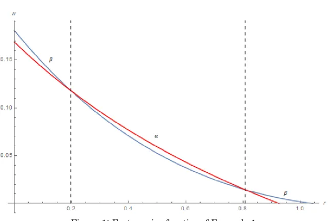
First, we con…rm the concepts used in this section. Let b 2 Rn+be a bundle of commodities
adopted as the numéraire. For the rate of pro…t such that r 2 [0; R ), where R denotes the maximum rate of pro…t attainable by technique 2 , the wage curve of technique measured by b can be de…ned as follows:
w (r) = 1
L [I (1 + r) A ] 1b.
w (r) is a function of r that corresponds to (A ; L ) for 2 . Furthermore, we de…ne the factor price frontier ! (r) as follows:
! (r) max
2 w (r) :
In other words, the factor price frontier is the outermost envelope of the wage curves, which implies that the cost-minimising technique for the given rate of pro…t is that by which the highest wage rate can be o¤ered (Kurz and Salvadori, 1995, p. 142).
4.1
Numerical Example
We consider the following numerical example:
Example 1: We suppose a two-class economy with two commodities. Commodity 1 has only one process: [a1; L1] =
2=5
2 ; 1 and commodity 2 has two alternative processes and : [a2 ; L2 ] = 1=40 1=10 ; 1 and [a2 ; L2 ] = 0:0001 113=232 ; 275 464 .
8 The technology available to
the whole economy are given as follows:
A = 2=5 1=40 0:0001 2 1=10 113=232 ; L = 1 1 275 464 . Therefore, we have [A ; L ] = 2=5 1=40 2 1=10 ; (1; 1) ; [A ; L ] = 2=5 0:0001 2 113=232 ; 1; 275 464 . Here, the set =f ; g is de…ned. We consider the wage curves of technique for 2 obtained by adopting a bundle of commodities b = 1
0 as the numéraire. Figure 1 depicts the wage curves and thus, the factor price frontier as their outermost envelope.
Insert Figure 1 here.
The intersection of the wage curves, called the switch points, are given by r t 0:197; 0:807. As the long-run competitive equilibrium technique (i.e. cost-minimising technique for given rate of pro…t), is chosen at r 2 [0; 0:197), is chosen at r 2 (0:197; 0:807), and is chosen again at r 2 (0:807; 1:04), where R = 1:04.9 Figure 1 shows that both reswitching
of technique and reverse capital deepening occur.10 Since technique , which is chosen in
r 2 [0; 0:197), is chosen again in r 2 (0:807; 1:04), the reswitching of technique occurs. Since the switch of technique from to at r t 0:8007 implies that technique with higher capital intensity is chosen despite the rise of the rate of pro…t, reverse capital deepening occurs. In the following part, we assume c = 0:7 and w = 0:3, unless otherwise stated.
4.1.1 Relationship between the rate of economic growth and that of pro…t in the case of (ILA, ILA)
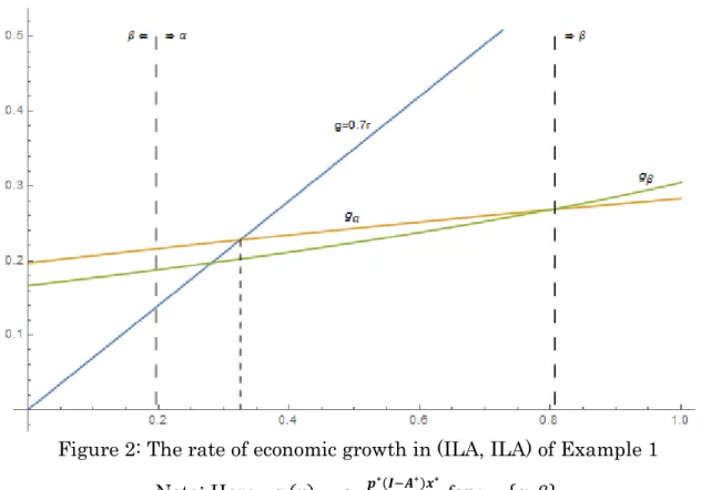
Under the above assumptions, we obtain the relationship between the rates of economic growth and pro…t, given by (15). Figure 2 shows the relationship under the technology given in Example 1.
Insert Figure 2 here.
In Figure 2, g and g denote the rate of economic growth as a function of the rate of pro…t in the DE when and , respectively, are activated as the long-run competitive equilibrium technique. The rate of economic growth as a function of the rate of pro…t in the PE is indicated by g = 0:7r, whichever is the long-run competitive equilibrium technique.
As con…rmed in Figure 1, technique is the long-run competitive equilibrium tech-nique for r 2 [0; 0:197) and thus, is chosen in the interval of the rate of pro…t. Note that 0:7r < 0:3 r + p A x1 g (r), where A = A , holds for r 2 [0; 0:197). Since we have a higher rate of economic growth in the steady state, as argued in Section 3.1.4, the DE is obtained under technique in the interval of the rate of pro…t. For r 2 (0:197; 0:807), as shown in Figure 1, the long-run competitive equilibrium technique is . Because of g (r) 0:3 r + 1
p A x , where A = A , the intersection between g = 0:7r and g = g (r)
is given by r t 0:325. Then, 0:7r 5 g (r) holds for r 2 (0:197; 0:325]. This result implies
9Note that each commodity has the same price at the switch points irrespective of whether it is produced
by any technique or any convex combination of techniques. See Kurz and Salvadori (1995, p. 142) and Pasinetti (1977, pp. 158–159).
10These phenomena are inconsistent with the principle of marginal productivity of capital. According
to the principle, there is a one-to-one correspondence between the rate of pro…t and the cost-minimising technique. The reswitching of technique means that one technique, which is chosen as the cost-minimising technique at the rate of pro…t, is also chosen at other rate of pro…t. Moreover, according to the principle, the capital intensity (value of capital per worker) is a monotonically decreasing function of the rate of pro…t. Reverse capital deepening (or capital reversing) means that the increase in the rate of pro…t raises the capital intensity. See, for example, Kurz and Salvadori (1995, pp. 147–149) and Pasinetti (1977, pp. 169–173) for details.
that the DE is obtained under technique for r 2 (0:197; 0:325]. For r 2 (0:325; 0:807), on the contrary, 0:7r > g (r) holds, implying that the PE is obtained under technique in the interval of the rate of pro…t. Furthermore, for r 2 (0:807; 1:04), the long-run com-petitive equilibrium technique is again. Recall that reswitching of technique and reverse capital deepening take place in the switching technique from to at r 0:807. For r 2 (0:807; 1:04), 0:7r > g (r) holds. This result means that the PE is obtained for in the interval of the rate of pro…t. Note that the relationship between the rate of economic growth and that of pro…t in the PE, represented by g = 0:7r, is unchanged even though the long-run competitive equilibrium technique changes from to .
Since the cost of production is always minimised at the switch points regardless of which technique or convex combination of existing techniques is used, as mentioned in footnote 9, the long-run competitive equilibrium is consistent with the multiple rates of economic growth at the switch points. However, it would be reasonable to suppose that the highest rate of economic growth is preferred. Then, the DE is obtained under technique at r 0:197and the PE at r 0:807.
Let (r) g (r)
w for 2 . From the de…nition of g = g (r), (r) denotes the ratio of
net output to capital when 2 is the long-run competitive equilibrium technique at r 2 [0; R ). Under the technology given in Example 1, 0:268 g (0:807) < g (0:807) 0:294.11
This result implies that (0:807) < (0:807). In other words, the ratio of net output to capital rises when the long-run competitive equilibrium technique switches from to at the switch point r 0:807. The movement of (r)around r 0:807is compatible with the principle of marginal productivity of capital. However, the movement of the capital intensity when the long-run competitive equilibrium technique switches from to at r 0:807 is inconsistent with the principle, since reverse capital deepening occurs. Figure 2 demonstrates that among two indexes characterising the technique in the neo-classical production function, one movement (ratio of net output to capital) is compatible with the principle but the other (capital intensity) is not. The result cannot be obtained by the model in which capital is treated as the primary factor of production. When capital is composed of a bundle of reproducible and heterogeneous commodities, the phenomena incompatible with the principle are not necessarily considered as paradoxical.
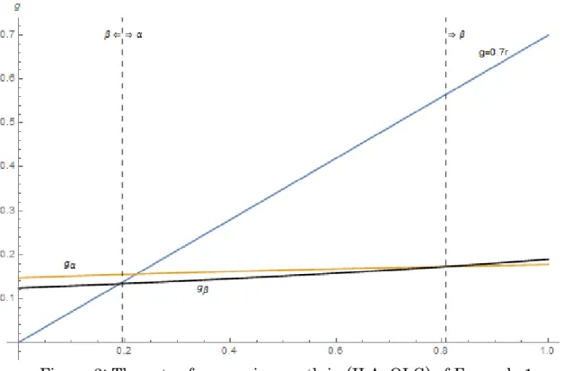
4.1.2 Relationship between the rates of economic growth and pro…t in the case of (ILA, OLG)
Next, we examine the case of (ILA, OLG) under the technology given in Example 1. Figure 3 shows the relationship between the rates of economic growth and pro…t, given by (21):
Insert Figure 3 here.
In Figure 3, similar to Subsection 4.1.1, g and g denote the the rate of economic growth as a function of the rate of pro…t in the DE when and , respectively, are utilised as the long-run competitive equilibrium technique. Note that g (r) is the worker’s saving rate
multiplied by the ratio of labour to capital (reciprocal of capital intensity) in this case. The rate of economic growth as a function of the rate of pro…t in the PE is given by g = 0:7r, which is the same function as that obtained in Subsection 4.1.1. This veri…es the result obtained in (15) and (21).
The intersection between g = g (r) and g = 0:7r is given by r 0:191. Therefore, the DE is obtained for r 2 [0; 0:191] and the PE for r 2 (0:191; 0:197) under technique . The DE is obtained for r 2 [0:197; 0:223] and the PE is obtained for r 2 (0:223; 0:807) under technique , where r 0:223 is the intersection between g = g (r) and g = 0:7r. For r 2 (0:807; 1:04), moreover, the PE is obtained under technique .
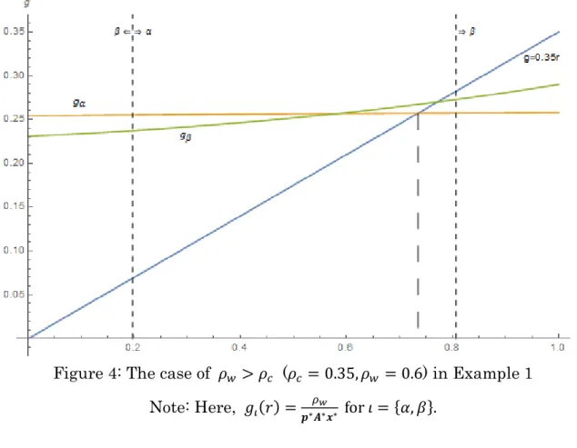
4.1.3 The case of w > c in (ILA, OLG)
As already pointed out in Subsection 3.4, (10) is an indispensable assumption to ensure the existence of the PE in the case of (ILA, ILA) but not in the case of (ILA, OLG). In this subsection, we examine the case of w > c in (ILA, OLG) by assuming the technology given
in Example 1 and w = 0:6; c = 0:35. This case is unrealistic but is a logical exercise to
test the working of the Pasinettian two-class model with a microfoundation of capitalist and worker.
Figure 4 shows the relationship between the rates of economic growth and pro…t in this case:
Insert Figure 4 here.
The …gure indicates that the DE is obtained under technique for r 2 [0; 0:197), and the DE is obtained under technique for r 2 [0:197; 0:735], where r 0:735 is the intersection between g = g (r) and g = 0:35r. Furthermore, the PE is certainly obtained under technique
for r 2 (0:735; 0:807) and under technique for r 2 [0:807; 1:04).
4.2
Short remarks of Section 4
In Section 4, we closely examine the results obtained in Section 3 by using the numerical examples. Although these examples may be speci…c, they provide useful insight of the analysis of the distribution of income and capital (wealth).
From Figures 2, 3, and 4, we observe that even when techniques switch from one to another, the relationship between the rates of economic growth and pro…t obtained in the PE, which is given by g = cr, is independent of the technology and the microfoundation
of the capitalist’s and worker’s behaviour. In addition, we observe from the …gures that the relationship obtained in the DE depends on the technology and the microfoundation of agents for the given rate of pro…t.
Although the movement of the capital intensity around the switch point exhibits para-doxical behaviour in Figure 2, that of the ratio of net output to capital is compatible with the principle of marginal productivity of capital. This interesting result is obtained only in the model in which capital is treated as a bundle of reproducible and heterogeneous commodities.
Moreover, the phenomena inconsistent with the principle of marginal productivity of capital are not necessarily considered as a paradox.
The fundamental cause of such paradoxical phenomena arising is our assumption that capital consists of a bundle of reproducible and heterogeneous commodities and not that our model lacks a continuous and di¤erentiable production function. Obviously, our assumption on capital is realistic. Burmeister (1981) shows that even when neo-classical well-behaved production functions are assumed, the possibility of paradoxical phenomena arising cannot be excluded if capital consists of reproducible and heterogeneous commodities. To exclude this possibility, a peculiar assumption which is unnecessary in the one-commodity model needs to be made.12
The rate of economic growth obtained in the PE is necessarily an increasing function of that of pro…t, irrespective of the microfoundation of agents and the technology. Although the relationships characterising the DE in the cases of both (ILA, ILA) and (ILA, OLG) are also an increasing function of the rate of pro…t in Example 1, we can easily …nd numerical examples in which the rate of economic growth is a decreasing function of that of pro…t in the DE, depending on the assumption of the microfoundation of the agents.13 Complicated
relationships between the rate of economic growth and income distribution can be obtained only by employing multi-sectoral models with capital as a bundle of reproducible and het-erogeneous commodities. In fact, we know little about the movement of g (r) for 2 unless the neo-classical production function is assumed, since it depends on the property of the technology and there are complicated e¤ects on the aggregation of income and capital when capital consists of a bundle of reproducible and heterogeneous commodities.
5
Concluding Remarks
In this study, we examine the distribution of income and capital (wealth) by a multi-sectoral two-class model with a microfoundation of capitalists and workers. The characteristic of our model is to treat capital as a bundle of reproducible and heterogeneous commodities. Clearly, capital in that sense, rather than capital as the primary factor of production, is a typical factor of production in modern capitalist economies. Our model can be considered as a summary of the Cambridge capital controversy in that it enables us to comprehensively analyse the major issues of the controversy (i.e. controversy about the Cambridge equation and the choice of technique) by using a single model. The aggregate macroeconomic model is used to address the former issue and the multi-sectoral model à la the Leontief–Sra¤a is used to address the latter.
12According to Burmeister (1981), this peculiar assumption is that the so-called real Wicksell e¤ect is
negative for all feasible r > 0:
n X i=1 pi(r) dki(r) dr < 0;
where pi(r) and ki(r) denote the relative price of commodity i and the per capita amount of the commodity
necessary as the capital input, respectively. As our analysis shows, it is not necessary to assume that the inequality is likely to be satis…ed.
13See Appendix A for a numerical example in which the rate of economic growth is a decreasing function
The movements of the ratio of net output to capital, the capital intensity, and the rate of pro…t (or wage rate) are important variables for analysis of the distribution of income and capital (wealth). According to the principle of marginal productivity of capital, the ratio of net output to capital declines when the wage rate rises. Stiglitz (2016) considers the recent rise in the US ratio of wealth to income without a substantial increase in the wage rate to be a paradox, and argues that the movement of the ratio cannot be explained by the standard neo-classical growth theory with the well-behaved production function.
We show that the movements of the ratio of net output to capital and the capital intensity when the rate of pro…t changes could be more complicated than those predicted by the models assuming the neo-classical well-behaved production function. This is because not only the quantities but also prices of capital change when the rate of pro…t changes if capital is treated as a bundle of reproducible and heterogeneous commodities. The changes in both quantities and prices generate the complicated e¤ects on the aggregation of income and capital. If capital is treated as the primary and homogeneous factor of production, as in the neo-classical production function, then the change in the rate of pro…t generates only a change in the quantities. According to the lesson of the Cambridge capital controversy, the phenomena indicated by Stiglitz are not necessarily a paradox, as we show in Sections 3 and 4. The growth models assuming the neo-classical well-behaved production function are not useful for predicting what happens to the steady states of the two-class economies on which C3 is imposed. This result implies that it is necessary to analyse the distribution of income and capital (wealth) by the models with capital as a bundle of reproducible and heterogeneous commodities.
Of course, our study leaves some open questions. We focus only on the properties of steady states. Signi…cant remaining questions are whether an economy starting from the initial value converges toward the steady state and, if it does, what equilibria it is likely to converge toward. Examination of these questions in the two-class model with capital as a bundle of reproducible and heterogeneous commodities remains as our future research agenda.
6
Appendix A
Here, we show the numerical example in which the rate of economic growth is a decreasing function of that of pro…t:
Example 2:14 We assume a two-class economy with two commodities. Commodity 1 has
two alternative processes and : [a 1; L 1] =
0
0:5 ; 1 , [a 1; L 1] =
0
0:125 ; 2 . In ad-dition, commodity 2 has only one process: [a2; L2] =
0:5
0 ; 1 . Therefore, the technology available in the economy as a whole is given as follows:
A= 0 0 0:5
0:5 0:125 0 ; L = 1 2 1 .
Then, we have
[A ; L ] = 0 0:5
0:5 0 ; (1; 1) ; [A ; L ] =
0 0:5
0:125 0 ; (2; 1) .
Here, the set =f ; g can be de…ned. Figure 5 depicts the wage curves of technique 2 and the factor price frontier. It demonstrates that neither reswitching of technique nor reverse capital deepening occur: the technique switches from to at r 0:143, and technique , which has lower capital intensity than technique , is chosen for r 2 [0:143; 3]. Note that the wage curve of technique is linear, since the so-called organic composition of capital is uniform in both sectors.
Insert Figure 5 here.
We assume that c = 0:7 and w = 0:3 as before. From (15) and (21), we obtain the
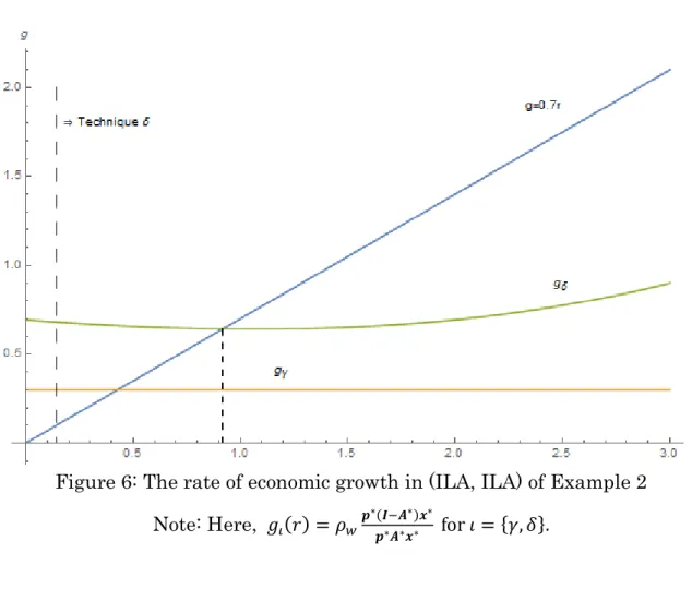
rate of economic growth as the function of the rate of pro…t in the case of (ILA, ILA) and (ILA, OLG). Figures 6 and 7 show the relationship between the rate of economic growth and that of pro…t in the former case and that in the latter case, respectively. Note that the price is normalised by w = 1 and the activity level by L x = 1 for 8r 2 [0; R).15 Figure 6
(ILA, ILA) shows that the DE obtained under technique is indicated by g for r 2 [0; 0:143); the DE obtained under technique is indicated by g for r 2 [0:143; 0:917], where r 0:917 is the intersection between g = 0:7r and g = g (r); and the PE is obtained under technique for r 2 (0:917; 3), where r = 3 is the maximum rate of pro…t obtainable under technique . Figure 7 (ILA, OLG) shows that the DE is obtained under technique for r 2 [0; 0:143); and the DE is obtained for r 2 [0:143; 0:994], where r 0:994 is the intersection between g = 0:7r and g = g (r); and the PE is obtained under technique for r 2 (0:994; 3).
Insert Figures 6 & 7 here.
Note that g in Figure 6 is constant independently of the level of r, since the ratio of net output to capital is constant irrespective of the level of r if the so-called organic composition of capital is uniform in all sectors (Pasinetti, 1977, p. 86). g in Figure 6 is not a monotonic function; the rate of economic growth is minimised at r 1:067. Therefore, we obtain the rate of economic growth as a decreasing function of the rate of pro…t for r 2 [0:143; 0:917]. In Figure 7, both g and g are decreasing functions of the rate of pro…t.
15Hosoda (1989) also draws the …gure in the case of (ILA, ILA) based on the same numerical example.
Although function (II) of Figure 6 in his study corresponds to g in our Figure 6, the form of his function (II) is di¤erent from that of our g . We assume that this is because he does not normalise the prices by w = 1, unlike in our study.
7
References
Baranzini, M. (1991) A theory of wealth distribution and accumulation. Oxford: Clarendon Press.
Baranzini, M., & Mirante, A. (2018) Luigi L. Pasinetti: An intellectual biography: Leading scholar and system builder of the Cambridge school of economics. Cham: Palgrave Macmil-lan.
Burmeister, E. (1981) Capital theory and dynamics. Cambridge: Cambridge University Press. Caggetti, M., & De Nardi, M. (2008) Wealth inequality: Data and models, Macroeconomic Dynamics, 12, 285–313.
Chappell, D., & Latham, R.W. (1983) The Pasinetti-Samuelson-Modigliani model as a two-person nonzero-sum di¤erential game, Keio Economic Studies, 20, 67–85.
Darity, W. A. (1981) The simple analytics of neo-Ricardian growth and Distribution. Amer-ican Economic Review, 71, 978–993.
De Nardi, M. (2015) Quantitative models of wealth inequality: A Survey. NBER Working Papers, 21106.
De Nardi, M., & Fella, G. (2017) Saving and wealth inequality, Review of Economic Dynam-ics, 26, 280–300.
Harcourt, G. (1972) Some Cambridge controversies in the theory of capital. Cambridge: Cambridge University Press.
Hosoda, E. (1989) Competitive equilibrium and the wage-pro…t Frontier. Manchester School, 57, 262–279.
Kaldor, N. (1956) Alternative theories of distribution. Review of Economic Studies, 23, 83–100.
Kaldor, N. (1961) Capital accumulation and economic growth, in Lutz, F. A., & Hague, D.C. (eds.) The theory of capital. London: Macmillan, 177–222.
Kurz, H., Salvadori, N. (1995) Theory of production: A long-period analysis. Cambridge: Cambridge University Press.
Mattauch, L., Edenhofer, O., Klenert, D., & Bénard, S. (2016) Distributional e¤ects of public investment when wealth and class are back, Metroeconomica, 67, 603–627.
Mattauch, L., Klenert, D., Stiglitz, J., & Edenhofer, O. (2017) Piketty meets Pasinetti: On public investment and intelligent machinery. Conference paper at Beiträge zur Jahrestagung des Vereins für Socialpolitik 2017: Alternative Geld- und Finanzarchitekturen - Session: Taxation II, No. B19-V2, ZBW - Deutsche Zentralbibliothek für Wirtschaftswissenschaften, Leibniz-Informationszentrum Wirtschaft, Kiel, Hamburg.
Meade, J. E. (1963) The rate of pro…t in a growing economy. Economic Journal, 73, 665–674. Meade, J. E. (1966) The outcome of Pasinetti-process: A note. Economic Journal, 76, 161– 165.
Meade, J.E., & Hahn, F. (1965) The rate of pro…t in a growing economy, Economic Journal, 75, 445–448.
Michl, T. (2007) Capitalists, workers and social security. Metroeconomica, 58, 244–268. Michl, T. (2009) Capitalists, workers, and …scal policy: A classical model of growth and distribution. Cambridge (Mass.): Harvard University Press.
Michl, T., & Foley, D. (2004) Social secutity in a classical growth model. Cambridge Journal of Economics, 28, 1–20.
Morishima, M. (1969) Theory of economic growth. Oxford: Clarendon Press.
Pasinetti, L. (1962) Rate of pro…t and income distribution in relation to the rate of economic growth. Review of Economic Studies, 29, 267–279; reprinted in Pasinetti (1974).
Pasinetti, L. (1964) A comment on professor Meade’s “Rate of pro…t in a growing economy.”, Economic Journal, 74, 488–489.
Pasinetti, L. (1966a) New results in an old framework: Comment on Samuelson and Modigliani. Review of Economic Studies, 33, 303–306.
Pasinetti, L. (1966b) The rate of pro…t in a growing economy: A Reply. Economic Journal, 76, 158–160.
Pasinetti, L. (1974) Growth and income distribution: Essays in economic theory. Cambridge: Cambridge University Press.
Pasinetti, L. (1977) Lectures on the theory of production. New York: Columbia University Press.
Pasinetti, L. (1983) Conditions of existence of a two class economy in the Kaldor and more general models of growth and income distribution. Kyklos, 36, 91–102.
Pasinetti, L. (2007) Keynes and the Cambridge Keynesians: A ‘revolution in economics’ to be accomplished. Cambridge: Cambridge University Press.
Pasinetti, L. (2012) A few counter-factual hypotheses on the current economic crisis. Cam-bridge Journal of Economics, 36, 1433–1453.
Piketty, T. (2014) Capital in the twenty-…rst century. Cambridge (Mass.): The Belknap Press of Harvard University Press.
Piketty, T. (2015) About Capital in the twenty-…rst century. American Economic Review, 105, 48–53.
Samuelson, P., & Modigliani, F. (1966a) The Pasinetti paradox in neoclassical and more general models. Review of Economic Studies, 33, 269–301.
Samuelson, P., & Modigliani, F. (1966b) Marginal productivity and the macro-economic theories of distribution: Reply to Pasinetti and Robinson. Review of Economic Studies, 33, 321–330.
Sasaki, H. (2018) Capital accumulation and the rate of pro…t in a two-class economy with optimization behavior. MPRA Paper, No. 88362.