Relation between torsion points and reduction of elliptic curves over number fields (Towards new development of mathematics via computational algebra system)

全文

(1)41. 数理解析研究所講究録第2012巻 2016年 41-65. Relation between torsion points and reduction of. elliptic. curves over. Masaya. number fields. Yasuda. Institute of Mathematics for. Industry,. Kyushu University Abstract This is a summary of our previous work on relation between torsion points and bad reduction primes of an elliptic curve E over a number. field. We. mainly. introduce. points of E of prime order. some. results. on. the non‐existence of. p if E has bad reduction. only. a. torsion. at certain. primes. related with p.. 1. Introduction. Let E be. elliptic curve over a number field K For a prime p the K‐rational p‐‐torsion points of E are the points of exact order p.in the Mordell‐Weil group E(K) In 1975, A. Ogg [Ogg75] first conjectured which groups can be \mathb {Q}‐rational torsion subgroups of an elliptic curve over \mathb {Q} In 1977, Mazur [Maz77, Maz78] proved Oggs conjecture and showed that any elliptic curve over \mathb {Q} cannot have a \mathb {Q}‐rational p\ovalbox{\t\smal RE‐torsion point for the primes p\geq 11 For quadratic fields, Kamienny J CT} and Kenku‐Momose [Kam92] [KM88] classified the possible torsion subgroups and showed that any elliptic curve over a quadratic field K has no K ‐rational p‐‐torsion points for the primes p\geq 17 For cubic fields, Parent [Par00, Par03] proved the same result on the non‐existence of p\mapst‐torsion points as in the case of o fields. it announced at the was 2010 quadratic Moreover, Algorithmic Number Theory Symposium (ANTS‐IX) [StolO] that Kamienny, Stein and Stoll proved that 17 is the largest prime dividing the order of the K‐rational torsion subgroup of an elliptic curve over any quartic field K. In addition to the above development on classification of possible p‐‐torsion points, the notion of reduction plays an important role in the theory of elliptic an. .. .. .. .. .. ,.

(2) 42. In this paper,. curves.. we are. interested in relation between the. (non‐)existence of. K ‐rational p\leftrighta‐torsion point of E and the primes at which E has bad reduction. r ow To investigate the relation, it is helpful to study the ramification of the extension a. K(E\lceil p]) torsion. K($\zeta$_{p}) where let K(E[p]) denote the field generated by the p‐ subgroup E[p] and $\zeta$_{p} a fixed primitive p‐th root of unity. Note that this over. ,. gives a Kummer extension of degree dividing p if E has a K‐rational p‐‐torsion point. Then the motivation of this paper is to study the relation extension. among the 1.. following. three mathematical. (Non‐)existence. 2. The. of. primes of K. a. K ‐rational. objects:. p‐‐torsion point of E. at which E has bad reduction. 3. Ramification of the extension. K(E\lceil p]). over. K($\zeta$_{p}). Agashe [Aga08] studied a part of the above relations. Specifically, he showed that if an elliptic curve over \mathb {Q} of square‐free conductor N (namely, a semi‐stable elliptic curve) has a \mathb {Q}‐rational p‐‐torsion point, for p\geq 5 then p divides either 6N or the order of the cuspidal subgroup of J_{0}(N)(\mathbb{C}) where let J_{0}(N) denote the Jacobian variety determined by the congruence subgroup $\Gamma$_{0}(N)\subset \mathrm{S}\mathrm{L}_{2}(\mathbb{Z}) T. Takagi [Tak12] gave an explicit formula for the order of cuspidal subgroups, and he combined his result with Agashes one to obtain a non‐existence result of a \mathb {Q} ‐rational p‐‐torsion point of semi‐stable elliptic curves over \mathb {Q} with certain conductor N This paper basically gives a summary of the authors previous work [Yas08, \mathrm{Y}\mathrm{a}\mathrm{s}\mathrm{l}2\mathrm{a}, \mathrm{Y}\mathrm{a}\mathrm{s}\mathrm{l}3\mathrm{a}, \mathrm{Y}\mathrm{a}\mathrm{s}\mathrm{l}3\mathrm{b}]. Especially, in this paper, we introduce an extension of Agashe‐Takagis non‐existence result. ,. ,. .. .. Notation. The. symbols \mathb {Z}, \mathbb{Q},. \mathbb{R} , and \mathb {C}. denote, respectively, the ring of. in‐. tegers, the field of rational numbers, the field of real numbers, and the field of complex numbers. For a prime p , the finite field with p elements is denoted by \mathb {F}_{p} Let $\zeta$_{p} denote a fixed primitive p‐th root of unity, and \dot{ $\mu$}_{p} the set of p‐th .. roots of. rational. unity. By \mathb {Z}_{p} and \mathb {Q}_{p}. ,. we. denote the. p‐‐adic integers and the p‐‐adic \mathcal{O}_{K} denote its ring of For a ring \mathcal{O}_{K} prime \mathfrak{p} of K let \mathcal{O}_{\mathfrak{p}. number field K , let. numbers, respectively. integers, and U_{K} the group of units in the be the completion of the ring \mathcal{O}_{K} at \mathfrak{p} and U_{\mathrm{p} denote the For. a. .. ,. We also define see. a. filtration. [Ser79, Chapter. We denote. IV. \{U_{\mathfrak{p} ^{(i)}\}_{i\geq 1} and. we. \mathcal{O}_{\mathfrak{p} . (e.g.. U_{\mathfrak{p} ^{(i)}=1+\mathfrak{p}^{i} \mathcal{O}_{\mathfrak{p} \supset U_{\mathfrak{p} \supset U_{\mathfrak{p} ^{(1)}\supset\cdots\supset U_{\mathfrak{p} ^{(i)}\supset\cdots. of the group. have. ,. group of units in. U_{\mathfrak{p} given by. by e_{\mathfrak{p} and f_{\mathfrak{p} the ramification index and the residue degree of \mathfrak{p}, respectively. Let v_{\mathfrak{p} be the normalized discrete valuation determined by \mathfrak{p} (then. we. have. v_{\mathfrak{p} (p)=e_{\mathfrak{p} )..

(3) 43. Preliminaries. 2. In this section, we give some basic results needed for our later discussions.. Elliptic. 2.1 Given. number field K and. a. having. with. curves. ‐torsion point. a. prime number p fix an elliptic point P Using the Weil‐pairing. a. K ‐rational 1 torsion. a. curves, which shall be. elliptic. on. curve. ,. E. over. K. .. e_{p}:E\lceil p]\times E\lceil p]\rightarrow$\mu$_{p}, define. we can. a. $\psi$. map. map. $\psi$ gives. an. E\lceil p]. :. \rightarrow$\mu$_{p} by. \mathrm{G}\mathrm{a}1(\overline{K}/K). absolute Galois group. exact sequence of. .. Q\mapsto e_{p}(P, Q). .. Let. G_{K} denote. Since the point P is rational. over. the. K , the. G_{K} ‐modules. 0\rightar ow \mathbb{Z}/p\mathbb{Z}\rightar ow E\lceil p]\rightar ow^{ $\psi$}$\mu$_{p}\rightar ow 0 \mathbb{Z}/p\mathbb{Z} is the constant G_{K} ‐module generated by P ing e_{p}(P, Q)=$\zeta$_{p} and.then the set \{P, Q\} forms a basis where. Q\in E\lceil p] satisfy‐ E\lceil p] as an \mathrm{F}_{p} ‐vector. Take. .. ,. (1). ,. of. space.. Lemma 2.1. Let. L=K(E\lceil p]). the p ‐torsion points. Proof.. Since. \mathrm{G}\mathrm{a}1(\overline{K}/L) contains. $\zeta$_{p}. of. ,. field. and hence. The action of. G_{K}. an. element. E[p] gives its associated. $\tau$\in G_{K}. tation induces the faithful exact sequence. (1),. the. generated by. .. for any element $\sigma$\in \mathrm{G}\mathrm{a}1(\overline{K}/L) Then L. ,. we. have. .. \square. have F\subseteq L.. we. Galois modulo p representation. \overline{ $\rho$}_{E,p}:G_{K}\rightar ow \mathrm{A}\mathrm{u}\mathrm{t}(E\lceil p])\simeq \mathrm{G}\mathrm{L}_{2}(\mathbb{F}_{p}) Given. K. is stable under the Galois group. $\zeta$_{\dot{p}. on. over. field F=K($\zeta$_{p}). $\sigma$($\zeta$_{p})=e_{p}( $\sigma$(P), $\sigma$(Q))=e_{p}(P, Q)=$\zeta$_{p}. the element. ,. denote the extension. E. Then L contains the. (2). .. \overline{$\rho$}_{E,p}($\tau$)\left(\b\mategin{ahrramy}{{lG }P\\mat Qh rm\e{nad}1{a(rLa/K)y}\r\igrhitg)=ht(_a{r$\otawu$\mat(Q)}^{h$r\mtau{G$(}P\)}mathrm{L}_{2}(\mathbb{F}_{p}). This represen‐. representation. representation. p. :. $\rho$ has the form. \left(\begin{ar y}{l 1&*\ 0&$\omega$ \end{ar y}\right). ,. where. .. By the. we. let. $\omega$:\triangle=\mathrm{G}\mathrm{a}1(F/K)\rightar ow \mathbb{F}_{p}^{\times} denote the. cyclotomic. character defined. by. $\sigma$($\zeta$_{p})=$\zeta$_{p}^{ $\omega$( $\sigma$)}. (3) for every $\sigma$\in\triangle..

(4) 44. Proposition 1. or. field. The. 2.2.. Kummer extension. a. \mathrm{G}\mathrm{a}1(L/F). The group. over. F of. degree dividing. under $\rho$. us. consider \triangle. a\in\triangle\subset \mathbb{F}_{p}^{\times}. .. acts. following. Proposition the extension. Here. result. L/F. give. some. as. on. either. a. on. extension. Kummer extension.. a. \square. \mathrm{G}\mathrm{a}1(L/F) by conjugation in \mathrm{G}\mathrm{a}1(L/K) by. cyclotomic. a\in \mathbb{F}_{p}^{\times}. gives. character. (_{0}^{1} k/a1). multiplication by a^{-1}. of unramified, p ‐part. \mathbb{Z}_{p}[\triangle] ‐module. elliptic. facts. is. an. .. Fix. we see. ,. Then. .. $\omega$. we can. the p‐‐part of the ideal class group of F :. is non‐trivial and. of. L/F. under the. \mathb {F}_{p}^{\times}. A_{F} denote the. 2.3. Let. Families of we. on. \left(\begin{ar y}{l 1&k\ 0&1 \end{ar y}\right) \mathrm{G}\mathrm{a}1(L/F). on. denote the $\omega$^{i} ‐eigenspace. 2.2. of. Since conjugating. a\in\triangle\subset \mathbb{F}_{p}^{\times}. obtain the. subgroup. as a. Therefore the field L is. .. p , and hence. We further consider the action of \triangle. that. of degree. F. isomorphic to the subgroup of \mathrm{G}\mathrm{L}_{2}(\mathb {F}_{p}) consisting. is. \left(\begin{ar y}{l 1&*\ 0&1 \end{ar y}\right). of all matrices of the form. Let. over. p.. Proof.. field. L is. curves. elliptic. curves. the ideal class group of F. If then where let R^{$\omega$^{ $\iota$} ,. A_{F}^{$\omega$^{-1} \neq 0. R.. with. p‐torsion. a. having. a. K ‐rational. point p‐‐torsion point. only for p=5 and 7. Let E be an elliptic curve over a number field K with a K ‐rational p‐‐torsion point P For p=5 and 7, there exists an element t\in K .. such that E is. isomorphic. to the. elliptic. curve. E_{t}^{(5)} y^{2}+(1-t)xy -- ty=x^{3} :. the Weierstrass. given by —. tx. 2. (if p=5 ),. E_{t}^{(7)} y^{2}+(1+t-t^{2})xy+(t^{2}-t^{3})y=x^{3}+(t^{2}-t^{3})x^{2} :. where the point P\in E. [Si186, Appendix. \mathrm{C} ] for. corresponds. details).. to. (0,0)\in E_{t}^{(p)}. E_{t}^{(p)}. \triangle(E_{t}^{(p)}=\left\{ begin{ar y}{l t^{5}.Q5(t)&\mathrm{f}\mathrm{o}\mathrm{r}p=5,\ t^{7}(t-1)^{7}\cdotQ_{7}(t)&\mathrm{f}\mathrm{o}\mathrm{r}p=7, \end{ar y}\right. where. we. set. \left\{ begin{ar ay}{l Q_{5}(X)=X^{2}-1 X-1,\ Q7(X)=X^{3}-8X^{2}+5X+1. \end{ar ay}\right.. (4). or. (if p=7 ),. (see [Kub76,. Then the discriminant of. equation. is. Table. (5) 3]. given by. or. ..

(5) 45. Modular. 2.2.1. For. an. Interpretation. odd prime number p , let. X_{1}(p). denote the modular. curve. associated to. the congruence subgroup $\Gamma$_{1}(p)\subset \mathrm{S}\mathrm{L}_{2}(\mathbb{Z}) According to [Si186, Appendix \mathrm{C} ], the modular curve X_{1}(p) is a smooth projective curve over \mathb {Q} , and it has (p-1) .. cusps. More. \displaystyle \frac{1}{2}(p-1). specifically, only. cusps. are. defined. In terms of modular curves, torsion point corresponds to curve. X_{1}(p). is. isomorphic. two cases, each. point. the function field. (in. this. setting, the correspondence. to. .. elliptic. one. K. K ‐rational p‐ having of X_{1}(p) In particular, the. curve over. K ‐rational. point the projective line \mathb {P}^{1} for one. [t, 1]\in \mathbb{P}^{1}. \mathbb{Q}(t). we. half of the cusps are defined over \mathb {Q} , but the other the maximal real subfield \mathbb{Q}($\zeta$_{p})\cap \mathbb{R} of \mathbb{Q}($\zeta$_{p}). over. maps to the. pair. a. .. cases. (E_{t}^{(p)}, P)\in X_{1}(p). where P is the K ‐rational p\overline{-} torsion. consider t. as an. indeterminate. in. [Fis00, Chapter 1]. tells. defined. point (0,0) of. element), namely,. \mathbb{P}^{1}\ni[t, 1]\mapsto(E_{t}^{(p)}, P)\in X_{1}(p) Furthermore, the result. p=5 and 7. In the. us. we. E_{t}^{(p)}. have. (6). .. that. over. we. have. (E_{t}^{(5)}, 2P)\simeq(E_{-1/t}^{(5)}, P) and (E_{t}^{(7)}, 2P)\simeq(E_{(t-1)/t}^{(7)}, P). (7). .. Fkom the. correspondence (6), the cusps of the curve X_{1}(p) correspond to the values t satisfying either \triangle(E_{t}^{(p)})=0 or t=\infty Therefore all the cusps of X_{1}(p) for p=5 and 7 are computable and shown in the below table: .. 2.2.2. Verdures Kummer generators. For any Kummer extension L/K($\zeta$_{p}) of satisfying both $\kappa$^{p}=a\in K($\zeta$_{p}) and. degree. p , there exists. an. L=K($\zeta$_{p}, $\kappa$)=K($\zeta$_{\mathrm{p} , $\varphi$_{\overline{a} ). Definition 2.4. We call such Kummer element. (resp.. an. Kummer. element $\kappa$\in L. generator). element $\kappa$\in L. .. (resp. $\kappa$^{p}=a\in K($\zeta$_{\mathrm{p}}) ) L/K($\zeta$_{p}). for the extension. .. \mathrm{a}.

(6) 46. Given. elliptic curve E over K having a K‐rational p‐‐torsion point, Verdure [Ver06] directly computed Kummer generators for the extension L=K(E[p]) over F=K($\zeta$_{p}) in cases p=3 5 and 7. His main idea for obtaining such a Kummer generator is to make use of Lagrange resolvents for the p‐th divi‐ sion polynomial associated to E For explicit Kummer generators obtained by Verdure, let us give the roots of the equation Q_{p}(X)=0 for p=5 and 7. an. ,. .. The. case. p=5. \left{\begin{ar y}{l Qs(X)&=\ $alph$_{5}&=\ $beta$_{5}&= \end{ar y}\ight. The. case. (X -\mathrm{a}_{5})(X-$\beta$_{5}). ,. 8+5$\zeta$_{5}+5$\zeta$_{5}^{4}, 3-5$\zeta$_{5}-5$\zeta$_{5}^{4}.. p=7. \left{bginary}{l Q_7}(X)&=-$\alph_{7})(X-$\beta_{7})(X-$\gam $_{7}),\ $alph_{7}&=1-2$\zeta_{7}-3$\zeta_{7}^2-3$\zeta_{7}^5-2$\zeta_{7}^6,\ $beta_{7}&=1-2$\zeta_{7}^2-3$\zeta_{7}^3-$\zeta_{7}^4-2$\zeta_{7}^5,\ $gam $_{7}&=1-3$\zeta_{7}-2$\zeta_{7}^3-2$\zeta_{7}^4-3$\zeta_{7}^6. \end{ary}\ight. Then. by. we are. Verdure. ready. (note. to introduce. that in. explicit. Kummer generators directly computed Theorem 5 and 6] he merely gives a criterion. [Ver06,. to decide whether all the p\leftrighta‐torsion r ow. Proposition 2.5 (see Theorem 5 \mathbb{Q}(t) of variable t For p=5 set .. points. are. and 6 of. rational. [Ver06]).. p=7. Let K be the. sion. function field. .. set. ,. a_{7}(t)=\displaystyle \frac{(t-$\alpha$_{7})(t-$\beta$_{7})^{2} {(t-$\gamma$_{7})^{3} \in K($\zeta$_{7}) Then, for. not):. ,. a_{5}(t)=\displaystyle \frac{t-$\alpha$_{5} {t-$\beta$_{5} \in K($\zeta$_{5}) For. or. E=E_{t}^{(\mathrm{p})}. L=K(E\lceil p]). Proof. See. the. ,. the element. over. a_{p}(t) gives. F=K($\zeta$_{p}) namely, ,. computational results. in the. a. .. Kummer generator. we. have. for the. L=F(\sqrt{a_{p}(t)}). proof of [Ver06, Theorem. exten‐. .. 5 and. 6]. for details. Note that all the computations in [Ver06] are performed using the software package MAGMA for arithmetic computations. Here we give only a.

(7) 47. sketch of his strategy; Let L=K(E\lceil p]) and F=K($\zeta$_{p}) By factoring the p‐th division polynomial associated to E into the product of irreducible polynomials, .. first find. we. Q\in E\lceil p] such that \{P, Q\} forms a basis of Ep\lceil J] as an \mathb {F}_{p^{-} P=(0,0) denotes the p‐‐torsion point of E Next we find a group \mathrm{G}\mathrm{a}1(L/F) satisfying $\sigma$(Q)=Q+P (see also [Ver06,. point. a. vector space, where. generator. $\sigma$. Corollary. 3. in the. .. Then, for \mathrm{r}\mathrm{c}. a. fixed number. i\in\{1, 2, . . . , p-1\}. ,. we. compute. =\displaystyle\sum_{k=0}^{\mathrm{p}-1}$\zeta$_{p}^{ik}$\sigma$^{k}(x_{Q})=\sum_{k=0}^{p-1}$\zeta$_{p}^{ik}x_{Q+kP}\inL,. where x_{R} denotes the x ‐coordinate of a point R of E Specifically, in the proof of [Ver06, Theorem 5 and 6], Verdure takes i=1 for p=5 and i=3 for p=7. .. By the above construction, the element. $\kappa$. clearly satisfies. $\sigma$($\kap a$)=\displaystyle\sum_{k=0}^{p-1}$\zeta$_{p}^{ik}x_{Q+(k+1)P}=$\zeta$_{p}^{-i}\sum_{k=0}^{p-1}$\zeta$_{p}^{i(k+1)}x_{Q+(k+1)P}=$\zeta$_{p}^{-i}$\kap a$. Therefore. we. have. $\sigma$($\kappa$^{p})=$\kappa$^{p} and L/F.. hence $\kappa$^{p}\in F , which. can. give. Kummer. a. generator for the extension. Non‐existence of. 3. Given. a. number field K and. between the non‐existence of. primes. a. a. \square. rational p‐torsion. point. prime number p\geq 5 we study the relation p‐‐torsion point of E over K and the ,. K ‐rational. a. at which E has bad reduction.. Definition 3.1. For any set S of primes of K , we say that an elliptic curve E over K has S ‐reduction if E has bad reduction only at the primes of S in other ,. words,. if E has. In the result. on. below,. first give points of an. we. p\overline{-} torsion. Theorem 3.2. real. good. (Theorem. place. p\geq 5 of K over p Set Let. reduction outside the primes of S.. be. a. a. main result. elliptic. 1.2 of. curve. [\mathrm{Y}\mathrm{a}\mathrm{s}\mathrm{l}2\mathrm{a}] ).. (cf. [Yas08, with. 0.1] for a everywhere good reduction):. Let K be. prime number such that. Theorem. number. field having a e_{\mathfrak{p}}<p-1 for the primes \mathfrak{p} a. .. S_{K,p}= { \mathrm{q} : prime of K Let E be. an. over a. prime. \ell|\ell\neq p. and. pf_{\mathfrak{q} \not\equiv\pm 1\mathrm{m}\mathrm{o}\mathrm{d} p }.. elliptic curve over K with S_{K,p} ‐reduction. If p does not divide the h_{F} of F=K($\zeta$_{p}) then E has no K ‐rational p ‐torsion points.. class number. ,.

(8) 48. The result of Theorem 3.2 in the. case. K=\mathbb{Q} shows. Theorem 3.3. (The. elliptic. \mathb {Q} only \mathb {Q} ‐rational p ‐torsion points.. curve over. then E has. no. case .. K=\mathbb{Q} of. Theorem. 3.2).. If E has bad reduction. The result of Theorem 3.3 includes. Let. at the. the. following. p=5. or. result:. 7. Let E be. an. primes P\not\equiv 0, \pm 1\mathrm{m}\mathrm{o}\mathrm{d} p,. Agashe‐Takagis. non‐existence result. [Aga08, Tak12], which enforces us to restrict the case where E is semi‐stable (see also Remark 3.7 below). Here we begin to prove Theorem 3.3. Specifically, present the following. we. 1. Let E be. two ways to prove Theorem 3.3:. elliptic. an. curve over. with. \mathb {Q}. a. \mathb {Q}‐rational p‐‐torsion point.. The. first way is to examine the finiteflat group scheme generated by the p‐ torsion subgroup E\lceil p] over the ring \mathbb{Z}[1/N] , where N is the product of the. primes. at which E has bad reduction. This. of Schoofs papers 2. In contrast,. given. an. elliptic. point, the second way is to extension. L=\mathbb{Q}(E\lceil p]). theory of Tate. Compared. curves. over. to. Agashe‐Takagis. to. The first. Here. we. Section. give. 2].. proof. the first. Let. us. part. curve. study. E. over. \mathb {Q} ‐rational p‐‐torsion primes of the Kummer particular, we make use of the \mathb {Q}. with. a. the ramified. F=\mathbb{Q}($\zeta$_{p}). .. In. proofs are so elementary and fundamen‐ knowledge about modular curves and forms.. way,. our. of Theorem 3.3. proof of Theorem 3.3, which basically taken from [\mathrm{Y}\mathrm{a}\mathrm{s}\mathrm{l}2\mathrm{a}, following well‐known lemma:. start with the. Lemma 3.4. Let E be a. on a. study such the ramification.. tal that it does not require any. 3.1. proof mainly relies. [Sch03, Sch05].. K ‐rational p ‐torsion. elliptic curve over point for p\geq 5 Let \mathrm{q} an. .. a. number. be. E has semi‐staule reduction at \mathrm{q}.. a. field K. Suppose prime of K with \mathrm{q} $\dag er$ p. .. E has Then. Proof. See the proof of [Fis00, Lemma 1.3] for details. Here we only consider case K=\mathbb{Q} ; Suppose E has additive reduction at a prime q\neq p Consider the filtration E(\mathbb{Q}_{q})\supset E_{0}(\mathbb{Q}_{q})\supset E_{1}(\mathbb{Q}_{q}) as described in [Si186, Chapter VII]. By the theory of formal groups, the multiplication by p is invertible on the the. group. .. E_{1}(\mathbb{Q}_{q}). .. The additive reduction tells. us. E_{0}(\mathbb{Q}_{q})/E_{1}(\mathbb{Q}_{q})\simeq \mathbb{F}_{q}^{+}. Tamagawa [E(\mathbb{Q}_{q}) : E_{1}(\mathbb{Q}_{q})] subgroup E(\mathbb{Q}_{q})[p] is trivial. This gives a E has a \mathb {Q} ‐rational p‐‐torsion point. This completes number. and the. Therefore the p‐‐torsion contradiction to the assumption that. is at most 4.. the. proof.. \square.

(9) 49. Let. p\geq 5 be a prime number and N a square‐free integer with p $\dag er$ N Let E elliptic curve over \mathb {Q} Assume that E has bad reduction only at the primes dividing N and E has a \mathb {Q}‐rational p‐torsion point P Let \mathcal{E} be the Néron model of E over \mathb {Z} By Lemma 3.4 and Grothendiecks semi‐stable reduction [Gro71, Theorem in Exp. IX], we see that \mathcal{E}[p] is a finite flat group scheme over the ring \mathbb{Z}[1/N] where let Glp] denote the kernel of multiplication by p for a group scheme G By [Maz77, Step 1 in Section 3], we have \mathbb{Z}/p\mathbb{Z}\subset \mathcal{E} where \mathbb{Z}/p\mathbb{Z} denotes the constant group scheme over \mathbb{Z}[1/N] generated by the point P. be. .. an. .. .. .. ,. .. ,. Lemma 3.5. The exact sequence. (1) of G_{\mathb {Q} ‐modules. induces. an. exact sequence. 0\rightarrow \mathbb{Z}/p\mathbb{Z}\rightarrow \mathcal{E}\lceil p]\rightarrow$\mu$_{p}\rightarrow 0 of finite flat. group schemes. (resp. diagonalizable) Proof. Let G be coker. over. \mathbb{Z}[1/N]. group scheme. ,. over. \mathbb{Z}/p\mathbb{Z} (resp. \mathbb{Z}[1/N]. where. $\mu$_{p} ) is. a. constant. finite flat group scheme over the ring \mathbb{Z}[1/N] defined by ( \mathbb{Z}/p\mathbb{Z}\rightar ow \mathcal{E}\lceil p]) It suffices to show that G is isomorphic to the diagonal‐ a. .. izable group scheme $\mu$_{p} over \mathbb{Z}[1/N] Since the group scheme G is étale over \mathbb{Z}[1/pN] , we can consider the group scheme G over \mathbb{Z}[1/pN] in terms of Ga‐ .. lois. modules, and hence G is isomorphic to the diagonalizable scheme $\mu$_{p} over \mathbb{Z}[1/pN] by the exact sequence (1). Next we consider the group scheme G over the ring \mathb {Z}_{p} Since any group scheme over \mathb {Z}_{p} is uniquely determined up to iso‐ morphism Uy its isomorphism type over \mathb {Q}_{p} (e.g., see [Tat97]), the group scheme G is isomorphic to the diagonalizable group scheme $\mu$_{p} over \mathb {Z}_{p} This shows that G is isomorphic to $\mu$_{p} over \mathbb{Z}[1/N] by [Sch03, Proposition 2.3]. \square .. .. Let. \mathrm{E}\mathrm{x}\mathrm{t}_{\mathb {Z}[1/N]}^{1}($\mu$_{p}, \mathb {Z}/p\mathb {Z}). denote the group of extensions of $\mu$_{p}. by \mathbb{Z}/p\mathbb{Z}. over. ring \mathbb{Z}[1/N] By the above lemma, we clearly have \mathcal{E}\lceil p] \in \mathrm{E}\mathrm{x}\mathrm{t}_{\mathb {Z}[1/N]}^{1}($\mu$_{p}, \mathb {Z}/p\mathb {Z}) In the case where N=\ell is a prime with \ell\neq p Schoof clarified the group \mathrm{E}\mathrm{x}\mathrm{t}_{\mathb {Z}[1/l]}^{1}($\mu$_{p}, \mathb {Z}/p\mathb {Z}) [Sch05, Corollary 4.2]. Based on [Sch05, Corollary 4.2], we shall give a key result to prove Theorem 3.3 as follows: the. .. ,. Proposition 3.6. Let p\geq 5 be a prime number and N a product of primes P\neq p with P\not\equiv\pm 1\mathrm{m}\mathrm{o}\mathrm{d} p Then the group \mathrm{E}\mathrm{x}\mathrm{t}_{\mathb {Z}[1/N]}^{1}($\mu$_{p}, \mathb {Z}/p\mathb {Z}) is trivial. .. Proof.. proof of [Sch05, Corollary 4.2]. Let \triangle= \triangle\rightar ow \mathbb{F}_{p}^{\times} denote the cyclotomic character (3). For let M^{$\omega$^{i} denote the $\omega$^{i} ‐eigenspace of M as in Proposition. The idea is based. \mathrm{G}\mathrm{a}1(\mathbb{Q}($\zeta$_{p})/\mathbb{Q}) any \mathbb{F}_{p}[ $\Delta$] ‐module. and let M,. $\omega$. :. on. the. ..

(10) 50. 2.3.. By. a. similar. proof of [Sch05, Proposition 4.1],. 0\rightar ow \mathrm{E}\mathrm{x}\mathrm{t}_{\mathb {Z}[1/N]}^{1}($\mu$_{p}, \mathb {Z}/p\mathb {Z}). we. get. an. exact sequence. (\mathbb{Z}[1/pN, $\zeta$_{p}]^{\times}/(\mathbb{Z}[1/pN, $\zeta$_{p}]^{\times})^{p})^{$\omega$^{2} \rightar ow (\mathb {Q}_{p}($\zeta$_{p})^{\times}/(\mathb {Q}_{p}($\zeta$_{p})^{\times})^{p})^{$\omega$^{2} \rightarrow. (8). We shall compute the group in the middle of the exact sequence (8). By the proof [Sch05, Corollary 4.2], we get the following exact sequence of $\omega$^{2} ‐eigenspaces. of. 0. where [. (\mathb {Z}[1/p, $\zeta$_{p}]^{\times}/(\mathb {Z}[1/p, $\zeta$_{p}]^{\times})^{p})^{$\omega$^{2}. \rightarrow. \displayst le\rightarow(\mathb {Z}[1/pN,$\zeta$_{p}]^{\times}/(\mathb {Z}[1/pN,$\zeta$_{p}]^{\times})^{p})^{$\omega$^{2}\rightarow(\bigoplus_{\mathrm{t}|N\mathb {F}_{p})^{$\omega$^{2}\rightarow0 runs over. the set of the. primes of \mathb {Z}[$\zeta$_{p}] lying over. N We .. identify. (9). ,. the Ga‐. lois group $\Delta$ with \mathb {F}_{p}^{\times} via the cyclotomic character $\omega$ By [Was82, Theorem 8.13], the \mathbb{F}_{p}[\triangle] ‐module \mathbb{Z}[1/p, $\zeta$_{p}]^{\times}/(\mathbb{Z}[1/p, $\zeta$_{p}]^{\times})^{p} is isomorphic to $\mu$_{p}\times \mathbb{F}_{p}[ $\Delta$/\{-1\rangle ]. .. So its $\omega$^{2} ‐eigenspace has module isomorphic to. dividing N assumption, .. \mathb {F}_{p} ‐dimension. \oplus_{l|N}\mathbb{F}_{p}[ $\Delta$/\langle P\rangle]. The $\omega$^{2} ‐eigenspace of the $\omega$^{2} ‐eigenspace of. 1. The module. ,. where \ell. \mathbb{F}_{p}[\triangle/\langle P\}]. \oplus_{1|N}\mathbb{F}_{p} is. runs over. permutation. the set of the. is trivial for which. \oplus_{\ell|N}\mathbb{F}_{p}[\triangle/(P\rangle ]. a. is trivial.. primes. $\omega$^{2}(\ell)\neq 1. .. By. This shows that. the group in the middle of the sequence (9) has dimension 1 over \mathb {F}_{p} Fur‐ thèrmore, since p\geq 5 , the $\omega$^{2} ‐eigenspace of \mathbb{Q}_{p}($\zeta$_{p})^{\times}/(\mathbb{Q}_{p}($\zeta$_{p})^{\times})^{p} has dimension .. By [Was82, Theorem 8.25], the $\omega$^{2} ‐eigenspace of the cyclotomic units is equal to the $\omega$^{2} ‐eigenspace of the local units. Therefore the $\omega$^{2} ‐eigenspace of the cyclotomic units in \mathbb{Z}[1/p, $\zeta$_{p}]^{\times} maps surjectively onto the $\omega$^{2} ‐eigenspace of \mathbb{Q}_{p}($\zeta$_{p})^{\times}/(\mathbb{Q}_{p}($\zeta$_{p})^{\times})^{p} It follows that the rightmost arrow in the sequence (8) is \square surjective. This completes the proof. 1.. .. Here. mainly based on the proof of [Maz77, Section 3]. Let p=5 or 7. Let E bè an elliptic curve over \mathb {Q} as in Theorem 3.3. Suppose E has a \mathb {Q}‐rational p\leftrighta‐torsion point P Set r ow E_{1}=E Since the exact sequence (1) of G_{\mathbb{Q} ‐modules is split by Lemma 3.5 and Proposition 3.6, there exists an elliptic curve E_{2} over \mathb {Q} and a \mathb {Q}‐isogeny E_{1}\rightarrow E_{2} with kernel $\mu$_{p} Then the image of the Galois submodule \mathbb{Z}/p\mathbb{Z} of E_{1}[p] gives a \mathb {Q}‐rational p‐‐torsion point in the elliptic curve E_{2} Continuing in this fashion, we obtain a sequence of \mathb {Q} ‐isogenies E_{1}\rightarrow E_{2}\rightarrow\cdots where each isogeny has kernel $\mu$_{p} and each curve E_{i} has a \mathb {Q}‐rational p‐‐torsion point. By Shafarevichs Theorem [Si186, Theorem 6.1], we see that E_{i_{0} \simeq E_{j\mathrm{o} for some we are. ready. to prove Theorem 3.3.. The idea is. .. .. .. .. ,.

(11) 51. Composing the above \mathb {Q}‐isogenies gives an endomorphism f : E_{i_{0}}\rightarrow over \mathb {Q} If P_{i_{0}}\in E_{i_{0}}(\mathbb{Q}) is the image of the starting p‐‐torsion point E_{i_{0}} P\in E(\mathbb{Q}) then by construction we have P_{i_{0} \not\in \mathrm{k}\mathrm{e}\mathrm{r}f Since \deg f is a power of p we see that f is a non‐scalar endomorphism. Therefore the elliptic curve E_{i_{0}} has complex multiplication. But this contradicts to Lemma 3.4 since any elliptic curve with complex multiplication cannot have semi‐staule reduction (e.g., see [Si186, Proposition 5.4 and 5.5] and [Si194, Corollary 6.4 ] )^{1} This completes the first proof of Theorem 3.3. \square i_{0}<j_{0}. .. defined. .. .. ,. ,. .. The second. 3.2 Here. we. Section P for. 3].. Theorem 3.3. proof of Theorem 3.3, which is taken from [\mathrm{Y}\mathrm{a}\mathrm{s}\mathrm{l}2\mathrm{a}, elliptic curve over \mathb {Q} with a \mathb {Q}‐rational r‐torsion point. the second. give. Let E be. p=5. proof of. an. To prove Theorem. 7.. or. 3.3,. it suffices to show that E has bad. reduction at p , or a prime \ell\equiv\pm 1\mathrm{m}\mathrm{o}\mathrm{d} p We note that E is isogeneous to an elliptic curve E over \mathb {Q} with a \mathb {Q}‐rational p‐‐torsion point such that \mathbb{Q}(E`\lceil p]) .. is. a. ramified extension of. reduction at the. same. \mathbb{Q}($\zeta$_{p}). primes,. of. we. degree. may. p. .. assume. Since both E and E have bad that. L=\mathbb{Q}(E\lceil p]). is. a. ramified. F=\mathbb{Q}($\zeta$_{p}) degree p. cyclotomic field F has class number 1, the extension L/F is rami‐ fied at some primes over a prime P By the proof of [Maz77, Step 3 in Section 3], we have \mathbb{Q}_{p}(E\lceil p])=\mathbb{Q}_{p}($\zeta$_{p}) if E has good reduction at p Hence we may assume P\neq p By the criterion of Néron‐Ogg‐Shafarevich [Si186, Theorem 7.1], we see that P is a prime of bad reduction for E Since E has semi‐stable reduction at P by Lemma 3.4, there exists an extension of M of degree 1 or 2 over \mathb {Q}_{\el } such that E is isomorphic to the Tate curve E_{q} over M where q denotes the Tate parameter (e.g., [Si194, Chapter V] for details). By the theory of Tate curves, Kummer extension of. of. Since the. .. .. .. .. ,. have. we. $\phi$:E(\overline{\mathb {Q} _{\el })\simeq\overline{\mathb {Q} _{\el }^{\times}/q^{\mathb {Z} . With this. $\phi$. ,. we. primitive pth is. a. .. Therefore. 1In order. [Tat74] any. .. $\phi$. :. hand, we. have. to lead this. that there is. elliptic. we. \simeq($\zeta$_{p}^{\mathb {Z} \cdot R^{\mathb {Z} )/q^{\mathb {Z} where R=q^{1/p}\in\overline{\mathbb{Q} _{\ell} is fixed have M(E[p])=M(q^{1/p}, $\zeta$_{p}) Since M(E|p]) a. ,. we. .. M($\zeta$_{p}) of degree p we see that q^{1/p}$\zeta$_{p}^{i}\not\in M for any i. $\zeta$_{p}\in M since the ptorsion point P is defined over \square [\mathbb{Q}_{\ell}($\zeta$_{p}) : \mathbb{Q}_{l}]=1 or 2, which means \ell\equiv\pm 1\mathrm{m}\mathrm{o}\mathrm{d} p. ,. have. contradiction, we further need the well‐known fact proved by Tate elliptic curve over \mathb {Q} with good reduction everywhere. In other words, \mathb {Q} with complex multiplication has always bad reduction somewhere.. no. curve over. E\lceil p]. Then. ramified extension of. On the other M. also have. root of q.

(12) 52. Remark 3.7. Here. [Aga08, Tak12] stable. The. we. briefly introduce. to prove Theorem 3.3. key. proof. in their. the. key result. in. Agashe‐Takagis. way. under the condition that E has semi‐. is the result of Theorem 1.1. proved by Agashe. [Aga08]. For the sake of simplicity, we here give an informal statement of his result (see [Aga08, Theorem 1.1] for details): Given an elliptic curve E over \mathb {Q} of square‐free conductor N Let .. r. be. a. prime dividing the order of the \mathb {Q}‐rational. subgroup E(\mathb {Q})_{\mathrm{t}\mathrm{o}\mathrm{r} Then the prime r divides either 6N or the order of the cuspidal subgroup C , where C is defined as the group of zero divisors on torsion. .. X_{0}(N)(\mathbb{C}). supported on the cusps Compared to our proofs, proof considerably tricky and it requires a lot of knowledge about the theory of modular forms. However, his proof is important in the literature, and it gives an interesting relation among torsion subgroups and cuspidal subgroups. In other words,, the (non‐)existence of a rational torsion point of an elliptic curve may be explained in terms of cuspidal subgroups. In fact, as mentioned in [Aga08, Section 1], he suspects E(\mathb {Q})_{\mathrm{t}\mathrm{o}\mathrm{r} \underline{\subseteq}C as long as N is square‐free. In particular, when N^{\mathrm{s} is prime, Mazur [\mathrm{M}\mathrm{a}\mathrm{z}7 ]\wedge proved that the modular. curve. his. two. C=J_{0}(N)(\mathbb{Q}). and hence the above relation holds in this. similar argument of the second. a. result of Theorem 3.2. field K. .. following. (a). case.. Proof of Theorem 3.2. 3.3. By. that. is. proof of Theorem 3.3, we can prove the generalization of Theorem 3.3 for a general number prime number and K a number field such that the. as a. Let. p\geq 5 be. two. conditions. a. are. satisfied:. p does not divide the class number. (b) e_{\mathfrak{p}}<p-1 Let E be. an. for all primes \mathfrak{p} of K. elliptic. curve over. h_{F} of. over. K with. F=K($\zeta$_{p}). ,. and. p. a. K ‐rational p\leftrighta‐torsion point. r ow. By. a. similar argument as in Section 3.2, we may assume that L=K(E\lceil p]) is a ramified extension over F òf degree p By the assumption (a), the extension L/F is ramified at some primes over a prime \mathrm{q} of K Let \mathfrak{p} be a prime of K .. .. over. p. .. By. the. order admits. a. assumption (b),. prolongation. any finite flat group scheme. over. the. over. K_{\mathfrak{p}. ring of integers of K_{\mathfrak{p} [Fon77,. of p‐‐power Théoreme. 3.3.3]. Therefore it follows from the proof of [Maz77, Step 3 in Section 3] that we K_{\mathfrak{p} (E\lceil p])=K_{\mathrm{p} ($\zeta$_{p}) if E has good reduction at \mathfrak{p} Hence we may assume \mathrm{q}|p Let P be the prime number satisfying \mathrm{q} \ell By a similar argument as in the previous subsection, we have [K_{\mathrm{q}}($\zeta$_{p}) : K_{\mathrm{q}}]=1 or 2, which means \square pf_{\mathrm{q} \equiv\pm 1\mathrm{m}\mathrm{o}\mathrm{d} p. have. .. .. ..

(13) 53. Elliptic. 4. p‐torsion. a. Given. having point. curves. prime number p\geq 5 and. a. a. both. S_{K,p} ‐reduction. number field K such that. e_{\mathfrak{p}}<p-1. and. for the. primes \mathfrak{p} of K over p Set F=K($\zeta$_{\mathrm{p}}) It follows from Theorem 3.2 that the class number h_{F} of F is divisible by p if there exists an elliptic curve E over .. .. having both S_{K,p} ‐reduction and a K‐rational p‐‐torsion point. This means of such a pair (E, K) tells us the p ‐divisibility of the class number h_{F} (note that there exist no such elliptic curves over \mathb {Q} since the class number of \mathbb{Q}($\zeta$_{p}) is equal to 1 for p=5 and 7). Here we give several examples of such pairs (E, K) only for p=5 and 7. 0urstrategy to construct such pairs K. that the existence. E=E_{t}^{(p)}. is to start with. K‐rational. taking an elliptic curve p‐‐torsion point P=(0,0). Proposition. 4.1. Let p=5. defined. in Section 2.2.. K. (5)) for S_{K,p} ‐reduction,. already defin ed Proof.. or. 7, which has. a. or. 7. Let. E=E_{t}^{(p)}, t\in \mathcal{O}_{K}. be. an. elliptic. curve over. Assume that the Weierstrass equation (4) (resp. E in the case p=5 (resp. the case p=7 ) is minimal. If. as. the equation E has. for p=5. .. then. Q_{p}(t)\in U_{K}. where the. in Subsection 2.2.. We consider. only. the. case. S_{K,p} ‐reduction. Then there exists 5t+1\in \mathcal{O}_{K} Since .. polynomial Q_{p}(X)\in \mathbb{Z}[X]. is. p=7 Assume that Q_{7}(t)\not\in U_{K} and E has prime P dividing the value Q_{7}(t)=t^{3}-8t^{2}+ .. a. \ell divides the minimal discriminant. \triangle(E)=t^{7}(t-1)^{7}\cdot Q_{7}(t). prime \mathrm{q} of K over P (it requires the assumption that \triangle(E) is minimal). Since E has S_{K,p} ‐reduction, we may assume P\neq 7 The solutions of the equation Q7(X) =X^{3}-8X^{2}+5X+1=0 define the extension field K($\zeta$_{7}+$\zeta$_{7}^{-1}) over K Now consider the diagram of E , the. curve. E has bad reduction at. a. certain. .. .. \mathrm{G}\mathrm{a}1(K($\zeta$_{7})/K). \lcorner+$\omega$. (\mathbb{Z}/7\mathbb{Z})^{\times}. \mathrm{e}\rightar ow. (\mathbb{Z}/7\mathbb{Z})^{\times}/\{\pm 1\},. \downar ow. $\sigma$\downar ow. \mathrm{G}\mathrm{a}1(K($\zeta$_{7}+$\zeta$_{7}^{-1})/K) where Let. \{s\}. .. $\omega$. is the. cyclotomic character defined by (3). s\in \mathrm{G}\mathrm{a}1(K($\zeta$_{7})/K) Note that. \Rightarrow \Rightarrow. we. have. and. $\sigma$. is the restriction map.. denote the Frobenius map satisfying \mathrm{G}\mathrm{a}1(K_{\mathrm{q} ($\zeta$_{7})/K_{\mathrm{q} )= $\omega$(s)=\ell f_{\mathrm{q} \in(\mathbb{Z}/7\mathbb{Z})^{\times} Then we obtain. Q_{7}(X)\equiv 0 mod \mathrm{q} has a solution X=t\in \mathcal{O}_{K}, Q_{7}(X)=0 has a solution X=t\in \mathcal{O}_{\mathrm{q}} by Hensels lemma,. $\sigma$(s)=1\in \mathrm{G}\mathrm{a}1(K($\zeta$_{7}+$\zeta$_{7}^{-1})/K)\Leftrightar ow\ell f_{\mathrm{q} \equiv\pm 1\mathrm{m}\mathrm{o}\mathrm{d} 7..

(14) 54. This is.a contradiction to the. We. assumption that E has S_{K,p^{\leftrightar ow}} reduction.. \square. ready to construct our desired pairs (E, K) Given a number field prime p=5 or 7, we only need to find t\in \mathcal{O}_{K} satisfying Q_{p}(t)\in U_{K}. Here we consider only the case of quadratic fields K=\mathbb{Q}(\sqrt{m}) where m is a square‐free integer. In this case, the assumption in Theorem 3.2 that e_{\mathrm{P}}<p-1 for the primes \mathfrak{p} of K over p is satisfied for p=5 and 7. Set t\cdot=a+b\sqrt{m}\in \mathcal{O}_{K} with 2a, 2b\in \mathbb{Z} Let 0\neq u=a^{2}-mb^{2}=\mathrm{N}\mathrm{m}_{K/\mathbb{Q}}(t)\in \mathbb{Z} denote the norm of t\in \mathcal{O}_{K} We consider each of the two cases p=5 and 7 as follows: K and. are. .. a. ,. .. .. The. 4.1. p=5. case. As described above, consider the condition. Q 5 (t)=t^{2}-11t-1\in U_{K}\Leftarrow\Rightarrow \mathrm{N}\mathrm{m}_{K/\mathbb{Q}}(t^{2}-11t-1)=\pm 1. \mathrm{N}\mathrm{m}_{K/\mathbb{Q}}(t^{2}-11t-1)=-4a^{2}-22(u-1)a+u^{2}+123u+1. Since. (10). is. ,. .. (10). the condition. to the condition. equivalent. X^{2}+11(u-1)X-u^{2}-123u-1=\pm 1 with X=2a\in \mathbb{Z}. .. Pell equation. Furthermore, the equation (11). can. (11). be transformed to the. A^{2}-5B^{2}=\pm 4. (12). with. \left\{ begin{ar ay}{l A=2X+1 (u-1)\in\mathb {Z},\ B=5(u+1)\in\mathb {Z}. \end{ar ay}\right. $\epsilon$=\displaystyle \frac{1+\sqrt{5} {2} integral Let. be. a. equation (12). solutions of the Pell. n=0 ,. 1, 2,. \cdots .. Since B\in 5\mathbb{Z}. \pm$\epsilon$^{5n} for. the elements. \mathbb{Q}(\sqrt{5}). fundamental unit of. n=0 ,. ,. we. 1, 2,. we can. construct. U_{K} for p=5 For example, .. \cdots. ,. Df the Pell equation. infinitely we. It is well known that the. given by the elements \pm$\epsilon$^{n} for (11) corresponds to namely, we have a correspondence are. note that the solutions of. \{t\in \mathcal{O}_{K}| Q5(t)\in U_{K}\}\leftrightarrow {Solutions Therefore. .. (12) given by \pm$\epsilon$^{5n} }.. (13). t\in \mathcal{O}_{K} satisfying Q_{5}(t)\in integral solution (A, B)=(-11, -5). many elements. have that. (12) corresponds. of. an. the element. -$\epsilon$^{5}=-\displaystyle \frac{1 +5\sqrt{5} {2}. .. Then the.

(15) 55. solution. (A, B)=(-11, -5) the condition (11).. further. corresponds. to. satisfying. An easy computation shows that. a. pair (X, u)=(11, -2). only the pairs. (X,u)=\left\{ begin{ar y}{l (10,-1),(12,-1),(1 ,-2),(2 ,-2),(12, 0),\ (-1 ,10),(10,-12),(13 ,-12),(2 ,12 ),\ (-1342,1 ),(0,-123),(1364,-123) \end{ar y}\right.. satisfy. (11) with |u|<1000 For each pair (X, u) we need to (a, b, m) and check whether the elliptic curve E_{t}^{(5)}, t=a+ K=\mathbb{Q}(\sqrt{m}) has S_{K,5} ‐reduction as in the following examples:. the condition. compute. a. .. ,. solution. b\sqrt{m}\in \mathcal{O}_{K}. over. Example 4.2. Here we give some examples of elliptic curves E_{t}^{(5)} over \mathbb{Q}(\sqrt{m}) having both S_{K,5} ‐reduction and a K‐rational 5‐torsion point.. (a, b, m)=(5,1,26) We see that elliptic E=E_{t}^{(5)}, t=a+b\sqrt{m} has good reduction everywhere over K=\mathbb{Q}(\sqrt{26}) (in fact, this curve appears in Cremonas table [Cre]). Therefore E has S_{K,5} ‐reduction. For. (X, u)=(10, -1). K=. the. For. have. a. solution. .. (X, u)=(11, -2). ,. we. have. a. solution. (a, b, m)=(\displaystyle \frac{11}{2}, \frac{1}{2},129). .. We. elliptic curve E=E_{t}^{(5)}, t=a+b\sqrt{m} has bad reduction only the primes of K=\mathbb{Q}(\sqrt{129}) over 2. Therefore E has S_{K,5} ‐reduction.. see. at. we. ,. curve. For. that the. (X, u)=(12,10). elliptic. curve. K=\mathbb{Q}(\sqrt{26}) 2,. a+b\sqrt{m}\in \mathcal{O}_{K}. we. we. have. a. solution. E=E_{t}^{(5)}, t=a+b\sqrt{m} over. 5, the elliptic. unlike the above two In Table. ,. (a, b, m)=(6,1,26). .. has bad reduction at the. curve. E does not have. Since the. primes of. S_{K,5} ‐reduction. curves.. triples (a, b, m) such that the elhptic curve E_{t}^{(5)}, t= K=\mathbb{Q}(\sqrt{m}) has S_{K,5} ‐reduction. Furthermore, for each. list. over. triple (a, b, m) we also list the class number h_{F}.\mathrm{o}\mathrm{f}F=K($\zeta$_{p}) which can be easily computed by [PARI] (version 2.4.1) (it is a free software library for arithmetic computations). As described in the first paragraph of Section 4, the class number h_{F} is divisible by p for all the triples (a, b, m) in Table 2. ,. 4.2. The. As in the. case. case. ,. p=7. p=5 consider the condition ,. Q_{7}(t)=t^{3}-8t^{2}+5t+1\in U_{K}\Leftrightarrow \mathrm{N}\mathrm{m}_{K/\mathbb{Q}}(t^{3}-8t^{2}+5t+1)=\pm 1. .. (14).

(16) 56. *. These. where. triples define elliptic. (see. Cremonas table. curves. [Cre]. with. good. reduction every‐. for list of such. elliptic curves). \mathrm{N}\mathrm{m}_{K/\mathbb{Q}}(t^{3}-8t^{2}+5t+1). A easy computation shows that. is. equal. to. 8a^{3}+(20u-32)a^{2}+(-16u^{2}-86u+10)a+(u^{3}+54u^{2}+4u+1) Therefore the condition. (14). to the condition. equivalent. is. X^{3}+(5u-8)X^{2}+(-8u^{2}-43u+5)X+(u^{3}+54u^{2}+4u+1)=\pm 1 with X=2a\in \mathbb{Z}. .. We. that. see. .. (15). only the pairs. (X, u)=(2,1) (6, -1) (7, -1) (7, -2) (8,5), (8,6), (9,7) ,. ,. ,. |u|<1000 In Table 2, we also list triples (a, b, m) such that the elliptic curve E_{t}^{(7)}, t=a+b\sqrt{m}\in \mathcal{O}_{K} over K=\mathbb{Q}(\sqrt{m}) has S_{K,7^{-}} reduction. As in the case p=5 the class number h_{F} of F=K($\zeta$_{7}) is divisible by 7 for all the triples (a, b, m) satisfy the. condition. (15). ,. with. .. ,. ..

(17) 57. Remark 4.3. The equation (15) defines a non‐singular projective curve C of genus 1. It follows from Siegels Theorem [Si186, Section 3] that the set C(\mathbb{Z}). of integral solutions is finite. Therefore, unlike in the case p=5 there are only finitely many elements t\in \mathcal{O}_{K} satisfying Q_{7}(t)\in U_{K} for p=7 Furthermore, we note that data of Table 2 are summarized again in Table 3 below \mathrm{i}_d}\mathrm{n} order ,. .. to show several unramified Kummer extensions. (we. also note that. elements of. we. F=K($\zeta$_{p}). for p=5 , 7 dont know whether the data of Table 2 can give all the over. C(\mathbb{Z}) ).. Ramification of Kummer extensions. 5. study the ramification of the Kummer extension L=K(E\lceil p]) an elliptic curve E over K having a K ‐rational p‐‐torsion F=K($\zeta$_{p}) The criterion of point. Néron‐Ogg‐Shafarevich [Si186, Theorem 7.1] implies that the ramification of the extension L/F is deeply related with the bad reduction primes of E Moreover, Kummer generators of L/F help us to study the ram‐ ification in more detail. Here we focus on Kummer extensions given by the p ‐torsion subgroup. of E=E_{t}^{(p)} for p=5 and 7, as defined in Subsection 2.2. We begin to introduce the following main result: In this section,. we. for. over. .. [\mathrm{Y}\mathrm{a}\mathrm{s}\mathrm{l}3\mathrm{b}] ). For p=5 or 7, set E=E_{t}^{(p)}, t\in \mathcal{O}_{K}. L=K(E\lceil p]) over F=K($\zeta$_{p}) has degree p then the is unramified outside the set of primes dividing Q_{p}(t)\in \mathcal{O}_{K}, L/F \dot{p} olynomial Q_{p}(X)\in \mathbb{Z}[X] is defined in Subsection 2.2.. Theorem 5.1. If. (Theorem. 1.1 of. the Kummer extension. extension. where the. Given. K(E[p]). an. and. elliptic. ,. curve. F=K($\zeta$_{p}). E=E_{t}^{(p)}, t\in \mathcal{O}_{K}. as. in Theorem 5.1.. over a. By. number filed K , set L=. the criterion of. Néron‐Ogg‐. primes dividing L/F t t-1 and in the and case p, p=5 (resp. the case p=7 ) Q_{p}(t) (resp. p, t, Q_{p}(t) ) since the discriminant \triangle(E) of E is equal to t^{5} Q5 (t) (resp. t^{7}(t-1)^{7}\cdot Q_{7}(t) ). Shafarevich,. the extension. must be unramified outside the. .. as. described in Section 2.2. In contrast, Theorem 5.1 further tells us that the L/F is unramified outside only the primes dividing Q_{p}(t)\in \mathcal{O}_{K} for. extension. p=5 and 5.1. 7.. Proof of Theorem 5.1. we shall give a proof of Theorem 5.1. Given an elliptic curve \mathcal{O}_{K} for p=5 or 7, our method is to study the ramification of. Here. E=E_{t}^{(p)},. t\in. the Kummer.

(18) 58. L=K(E[p]) over F=K($\zeta$_{p}) usíng Verdures explicit Kummer gen‐ a_{p}(t) given in Proposition 2.5. To prove Theorem 5.1, it only suffices to show that the Kummer extension L/F is unramified at the primes \mathfrak{P} of F satisfying v_{i}\mathrm{p}(Q_{p}(t))=0 ; this condition means that the value Q_{p}(t) is not di‐ extension. erators. visible. by \mathfrak{P} Before giving. a. .. proof,. give the following well‐known result of. we. ramification in Kummer extensions of prime Lemma 5.2. Let F be let. L=F($\varphi$_{X}). (i) If \mathfrak{Q}. is. a. be. number. a. degree.. field containing the p‐th roots of unity, field for some x\in F.. prime of F. dividing. not. p , then. only if v_{\mathfrak{Q} (x)\equiv 0\mathrm{m}\mathrm{o}\mathrm{d} p.. (ii). Let. be. \mathfrak{P}. Assume exists. an. x. L/F. is. unramífied. at \mathfrak{Q}. if. and. prime of F dividing. a. x\in U_{\mathfrak{P}. generator. and. Kummer extension. a. is. .. Then. L/F to. congruent. element. y\in U_{\mathfrak{P}. p with the ramification index e=e_{\mathfrak{P}}. unramified at \mathfrak{P} if and only if the Kummer a p‐th power modulo \mathfrak{P}^{ep/(p-1)} namely, there. is. ,. such that. x\equiv y^{p}\mathrm{m}\mathrm{o}\mathrm{d} \mathfrak{P}^{ep/(p-1)}\Leftar ow\Rightar ow x\cdot y^{-p}\equiv 1\mathrm{m}\mathrm{o}\mathrm{d} \mathfrak{P}^{ep/(p-1)}. Proof. See [CF67, and Exercise Then let. below. us. Exercise or. [Sai97,. 2.12]. The. Let \mathfrak{Q} be. a. proof of (i), and also [Was82, for a proof of (ii).. prove Theorem 5.1 for each of the two. case. Lemma 9.1. 8.38]. taken from. [\mathrm{Y}\mathrm{a}\mathrm{s}\mathrm{l}3\mathrm{b}. ,. cases. p=5. \square. and 7 in the. Section 3. p=5. not dividing 5, and assume v_{\mathfrak{Q}}(Q_{5}(t))= O. In this v_{\mathfrak{Q}}(a_{5}(t))=v\mathfrak{Q}(t-$\alpha$_{5})-v_{\mathfrak{Q}}(t-$\beta$_{5})=0 since the prime \mathfrak{Q} neither t-$\alpha$_{5} nor t-$\beta$_{5} due to the assumption v_{\mathfrak{Q}}(Q_{5}(t))=0 (we. we. divides. for. Theorem. (the proof is basically. 5.1.1. case,. 9.3]. a. prime of F. have. remark that two elements t-$\alpha$_{5} and t-$\beta$_{5} are in the ring \mathcal{O}_{F} and we have v_{5\supset}(t-$\alpha$_{5}) , v\mathfrak{Q}(t-$\beta$_{5})\geq 0 due to the assumption t\in \mathcal{O}_{K} ). Since the Kummer. generator. a_{5}(t). is not divisible. Kummer extension L=F. by \mathfrak{Q}. (\sqrt[5]{} (t)) a5. ,. it follows from Lemma 5.2. over. F is unramified at any. (i). that the. prime \mathfrak{Q} of. F. dividing 5 with v_{\mathfrak{Q}}(Q_{5}(t))=0. only suffices to consider the primes \mathfrak{P} of F dividing 5. As in the above, assume v_{\mathfrak{P}}(Q_{5}(t))= O. In this case, the prime \mathfrak{P} is over the prime \mathfrak{P}0=(1-$\zeta$_{5}) of the cyclotomic field \mathbb{Q}($\zeta$_{5})\subset F which is the only one prime over 5. The assumption v_{\mathfrak{P}}(Q5(t))=0 shows v_{i}\mathrm{p}(a5(t))=0 by the same argument as not. Then it. ,.

(19) 59. in the above. paragraph, and hence we have a5 (t)\in U_{\mathfrak{P}} To study the ramification L/F for the prime \mathfrak{P} over 5, we further need to .. of the Kummer extension consider which that purpose, a5. subgroup U^{(i)} of U_{\mathrm{a}\mathrm{s} ,. .. (t)-1=\displaystyle \frac{$\beta$_{5}-$\alpha$_{5} {t-$\beta$_{5} =\frac{-5(1+2$\zeta$_{5}+2$\zeta$_{5}^{4}) {t-$\beta$_{5} =\frac{-5(1-$\zeta$_{5})^{2}($\zeta$_{5}+$\zeta$_{5}^{2}) {t-$\beta$_{5} v_{i}\displaystyle \mathrm{p}(a_{5}(t)-1)=e\prime \mathrm{p}+\frac{e_{\mathfrak{P} }{2}=\frac{3e_{\mathfrak{P} }{2}. From this equation, we clearly have $\zeta$_{5}+$\zeta$_{5}^{2} of the field \mathbb{Q}($\zeta$_{5}) is not divisible. element. 0 due to the. by \mathfrak{P}0=(1-$\zeta$_{5}). i_{0}>\displaystyle\frac{pe_{\mathfrak{P} {p-1}. prime \mathfrak{P} dividing proof of Theorem 5.1.2. The. case. 5 with. v_{\mathfrak{P}}(Q_{5}(t))=0 by. 5.1 in the. case. L/F. Lemma 5.2. since the. and. U_{\mathfrak{P} ^{(i_{0}). subgroup. for p=5 , the Kummer extension. (16). .. v_{i}\mathrm{p}(t-$\beta$_{5})= v_{\mathfrak{P} (5)=e_{\mathfrak{P} ). Hence. also note that. v_{\mathfrak{P}}(Q_{5}(t))=0 (we. assumption. the Kummer generator a5 (t) is included in the. Since. generator a_{5}(t). For. contains the Kummer. consider. we. for. i_{0}=\displaystyle\frac{3e_{\mathfrak{P} {2}.. is unramified at any. (ii).. This. completes. the \square. p=5.. p=7. By a similar argument in the case p=5 it only suffices to consider the primes \mathfrak{P} dividing 7. Assume v_{\mathfrak{P}}(Q_{7}(t))= O. Then the prime \mathfrak{P} is over the prime \mathfrak{P}0= (1— $\zeta$7) of the cyclotomic field \mathbb{Q}($\zeta$_{7}) which is the only one prime over 7. The assumption v_{ $\zeta$}\mathrm{p}(Q_{7}(t))=0 tells us that we have v_{\mathfrak{P}}(a_{7}(t))=0 and hence a_{7}(t)\in U_{i}\mathrm{p} (the assumption t\in \mathcal{O}_{K} is necessary for this fact). As in the ,. ,. ,. argument of the. case. p=5. ,. we. need to consider which. generator a_{7}(t) By using the easily compute following:. contains the Kummer can. .. U_{\mathfrak{P} ^{(i)}. of U_{i}\mathrm{p} subgroup library [PARI], we. the software. a_{7}(t)-1 = \displaystyle \frac{(t-$\alpha$_{7})(t-$\beta$_{7})^{2}-(t-$\gamma$_{7})^{3} {(t-$\gamma$_{7})^{3} =\frac{A(t^{2}+Bt+C)}{(t-$\gamma$_{7})^{3}. (17). where. Note that. \left{\begin{ar y}{l A=&7(1+2$\zeta$_{7}^2+$\zeta$_{7}^3+$\zeta$_{7}^4+2$\zeta$_{7}^5)\mathrm{w}\mathrm{i}\mathrm{t}\mathrm{}v_{\mathfrk{P}0(A)=8,\ B=&-52$\zeta$_{7}^2-$\zeta$_{7}^5,\ C=&10+8$\zeta$_{7}^2+4$\zeta$_{7}^3+4$\zeta$_{7}^4+8$\zeta$_{7}^5. \end{ar y}\right.. we. have. v_{\mathfrak{P}}(t-$\gamma$_{7})=0 by. v_{\mathfrak{P}}(t^{2}+Bt+C)\geq 0 t\in \mathcal{O}_{K}). .. since. From the above. the. assumption v_{\mathfrak{P}}(Q_{7}(t))=0 and also requires the assumption ,. t^{2}+Bt+C\in \mathcal{O}_{F} (it. consideration,. v_{\mathfrak{P} (a7 (t)-1 ). we. have. \displaystyle \geq Vap(A)=\frac{8e_{\mathfrak{P} {6}=\frac{4e_{\mathfrak{P} {3}. (18).

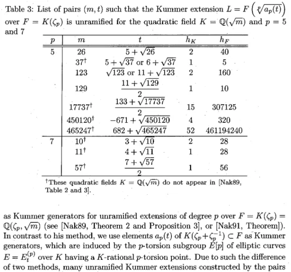
(20) 60. since. v_{\mathfrak{P} (\displaystyle \mathfrak{P}_{0})=\frac{e_{\mathfrak{P} {6}. due to that the extension. to 6. Hence the Kummer. i_{0}=\displaystyle\frac{4e_{\mathfrak{P} {3}. .. Since. i_{0}>\displaystyle\frac{pe_{\mathfrak{P} {p-1}. F is unramified at any 5.2 (ii). This completes the over. 5.2 Let his. a_{7}(t). generator for. degree. \mathbb{Q}($\zeta$_{7}). is included in the. p=7 the Kummer ,. \mathb {Q}. case. is. equal. U_{\mathfrak{P}^{(i_{0})\sim. for. L=F(\sqrt[7]{a_{7}(t)}). v_{\mathfrak{P}}(Q_{7}(t))=0 by. Theorem 5.1 in the. Unramified Kummer extensions. over. subgroup. extension. prime \mathfrak{P} dividing 7 with. proof of. of. Lemma \square. p=7.. generated. from. a_{p}(t). K=\mathbb{Q}(\sqrt{m}) be a quadratic field, where m is a square‐free integer. In papers [Nak89, Nak91], Nakagoshi gives an explicit condition for when a. fundamental unit of quadratic fields gives an unramified Kummer extension F=K($\zeta$_{p}) of degree p , and he also gives some examples of such unramified. over. p=3 5, 7 and 13 in [Nak89, Table 2 and 3]. In contrast to his examples, we give unramified Kummer extensions over the same field F generated from the Kummer generators a_{p}(t) given in Proposition 2.5 for p=5 and 7. For that purpose, we need to find elements t\in \mathcal{O}_{K} with Q_{p}(t)\in U_{K} by Theorem 5.1. These elements t\in \mathcal{O}_{K} have already been found in Section 4 (see also Proposition 4.1). In fact, some pairs (m, t) satisfying our desired condition for K=\mathbb{Q}(\sqrt{m}) are shown in Table 2. Hence we can give several unramified Kummer extensions over F generated from the Kummer generators a_{p}(t) for p=5 and 7, which we summarize in Table 3. As in Table 2, the class number h_{F} of F in Table 3 is divisible by p and hence the p\leftrightar ow part A of the ideal class group of F is not equal to zero (the class numbers h_{K} and h_{F} in Table 3 are computed by using [PARI]). Furthermore, since these fields F are constructed by the r‐torsion subgroup of elliptic curves, we have A_{F}^{$\omega$^{-1} \neq 0 by Proposition 2.3 (cf. only the content in Section 4 cannot show such the result because we cannot determine by Theorem 3.2 whether the Kummer Kummer extensions for. extension. ,. E_{t}^{(p)} is unramified not). Furthermore, Herbrands K=\mathbb{Q} for the primes p\geq 5 since A_{F}^{$\omega$^{-1} =0 in the. generated from. Theorem shows that. or. case. the Bernoulli number B_{2} is. equal. hand, the data in Table A_{F}^{$\omega$^{-1} \neq 0 for p=5 and 7. the other. to. 3. \displayte\frac{1}6 (see [Was82,. Section. give quadratic fields. 6.3]. for. details).. On. K=\mathbb{Q}(\sqrt{m}) satisfying. Our method to construct unramified Kummer extensions is quite different Nakagoshis one. In fact, he uses fundamental units of quadratic fields. from. \mathbb{Q}(\sqrt{m}). and. \mathbb{Q}(\sqrt{mp^{*}}). with. p^{*}=(-1)^{(p-1)/2}\cdot p.

(21) 61. Table 3: List of pairs over. F=K($\zeta$_{p}). (m, t). such that the Kummer extension. is unramified for the. L=F(\sqrt{a_{p}(t)}). quadratic field K=\mathbb{Q}(\sqrt{m}) and p=5. and 7. tThese quadratic fields K=\mathbb{Q}(\sqrt{m}) do. Table 2 and. not appear in. 3].. [Nak89,. Kummer generators for unramified extensions of degree p over F=K($\zeta$_{p})= \mathbb{Q}($\zeta$_{p}, \sqrt{m}) (see [Nak89, Theorem 2 and Proposition 3], or [Nak91, Theorem| ). as. In contrast to his. method,. generators, which. E=E_{t}^{(p)}. over. K. are. we use. induced. having. a. by. elements the. K ‐rational. of two. methods,. (m, t). in Table 3 do not appear in. Example. 5.3. In the. p=5. 6+\sqrt{37} we. we. ,. of. K($\zeta$_{p}+$\zeta$_{p}^{-1})\subset F. following,. rtorsion point.. [Nak89,. we. take. E=E_{t}^{(5)}. by. $\epsilon$. .. Table 2 and. describe. by. our. some. curves. by the pairs. 3].. typical examples of. unrami‐. method:. (m, t)=(37,6+\sqrt{37}). from Table 3. Then the element. quadratic field K=\mathbb{Q}(\sqrt{37}) which equation (4) of the elliptic curve given by (note that we have $\epsilon$^{2}=12 $\epsilon$+1 ). Then the Weierstrass. for t= $\epsilon$ is. Kummer. Due to such the difference. is the fundamental unit of the. denote. as. p‐‐torsion subgroup E\lceil p] of elliptic. many unramified Kummer extensions constructed. fied Kummer extensions constructed For. a_{p}(t). y^{2}+(1- $\epsilon$)xy- $\epsilon$ y=x^{3}- $\epsilon$ x^{2},. ,.

(22) 62. and this. good reduction everywhere over \mathbb{Q}(\sqrt{37}) since its dis‐ is equal to $\epsilon$^{6} (the curve E is isomorphic over \mathbb{Q}(\sqrt{37}) to Shimuras has. curve. criminant. [Kag98]. since the. j ‐invariant of E is equal to 2^{12} ). This [Cre]. Furthermore, the Kummer. curve. B37 given. curve. is alsó included in Cremonas table. a5(t). generator. in. for t= $\epsilon$ is. easily computed. as. a_{5}(t)=$\epsilon$^{-1}(10 $\epsilon \eta$-4 $\epsilon$+55 $\eta$+90). \displaystyle \frac{-1+\sqrt{5} {2}. where $\eta$ denotes the fundamental unit. a_{5}(t). is in the. quartic field. \mathbb{Q}(\sqrt{5};\sqrt{37}). for the unramified Kummer extension. of. and it gives. ,. L=K(E[5]). \mathbb{Q}(\sqrt{5}) a. .. The element. Kummer generator. over. F=K($\zeta$_{5}). .. p=7 we take (m, t)=(10,3+\sqrt{10}) from Table 3. As in the above example, the element 3+\sqrt{10} is the fundamental unit of the quadratic field K=\mathbb{Q}(\sqrt{10}) which we denote by $\epsilon$ Then the Weierstrass equation For. ,. .. ,. (5). of the. elliptic. curve. $\epsilon$^{2}=6 $\epsilon$+1). E=E_{t}^{(7)}. for t= $\epsilon$ is given. by (note that. we. have. y^{2}-5 $\epsilon$ xy-(31 $\epsilon$+5)y=x^{3}-(31 $\epsilon$+5)x^{2}, and this. curve. has. good. reduction. 2 and 3 since its discriminant is. Then. we can see. \mathbb{Q}($\zeta$_{7}+$\zeta$_{7}^{-1}, \sqrt{10}). equal. that the element ,. Kummer extension. and it gives. a. L=K(E[7]). over. \mathbb{Q}(\sqrt{10}) outside the primes over -$\epsilon$^{9}( $\epsilon$-1)^{7}=-$\epsilon$^{9}(2+\sqrt{10}). to. a_{7}(t). .. for t= $\epsilon$ is included in the field. Kummer generator for the unramified. over. F=K($\zeta$_{7}). .. References [Aga08]. A.. Agashe, Rational. torsion in. arXiv preprint arXiv:0810.5181. [CF67]. J.W.S. Cassels and A.. Press,. [Cre]. curves. and the. cuspidal subgroup,. (2008).. Frölich, Algebraic Number Theory, Academic. 1967.. J. Cremona over. elliptic. (compiled), Elliptic. quadratic fields,. curves. available at http:. with. everywhere good. reduction //homepages.warwick.ac. \mathrm{u}\mathrm{k}/. Staf \mathrm{f}/\mathrm{J} E. Cremona//e cegr/ecegrqf. html. .. [FisOO]. T. A.. Fisher, On 5 and 7 descents for elliptic University of Cambridge (2000).. curves, PhD. Thesis,. The.

(23) 63. [Fon77]. J.‐M.. [Gre89]. C.. [Gro71]. A.. [Kag98]. T.. Fontaine, Groupes p ‐divisible 48, Soc. Math. France, Paris (1977).. sur. les corps. locaux, Astérisque. Greither, Unramified Kummer extensions of prime Manuscripta Math. 64(3) (1989), 261‐290.. power. 47‐. degree,. Grothendieck, Modèles de Neron et monodromie, Exp IX in Groupes de monodromie en géométrie algébrique, SGA 7, Part I, Lecture Notes in Mathematics 288 (1971) Springer‐Verlag, Berlin‐Heidelberg‐New York. Kagawa,. duction. [Kam92]. S.. over. Determination. \mathbb{Q}(\sqrt{37}). ,. of elliptic. Acta Arith. 89. curves. (1998). with. everywhere good. re‐. 253‐269.. Kamienny, Torsion points on elliptic curves and forms, Invent. Math. 109 (1992), 221‐229.. q ‐coeficients. of. modular. [KM88]. Momose, Torsion points on elliptic curves defined quadratic fields, Nagoya Math. J. 109 (1988), 125‐149.. M. Kenku and F.. over. [Kub76]. Kubert, Universal bounds. D.. London Math. Soc. 33. [Maz77] 47. B.. Mazur, Modular. (1977),. [Maz78]. B.. (1976), curves. on. the torsion. of elliptic. curves, Proc.. 193‐237.. and the Eisenstein. ideal, IHES Publ. Math.. 33‐186.. Mazur, Rational isogenies of prime degree, Invent. Math.. 44. (1978),. 12‐162.. [Nak89]. Nakagoshi, On the unramified extensions of the prime cyclotomic field and its quadratic extensions, Nagoya Math. J. 15 (1989) 151‐. N.. number 164.. [Nak91]. Nakagoshi, On the unramified Kummer extensions of quadratic ex‐ of the prime cyclotomic number field, Arch. Math. (Basel) 57(6). N.. tensions. (1991). [Kra96]. A.. [Ogg75]. A.. 566‐570.. Kraus,. Courbes elliptiques semi‐stables Theory 60, (1996), 245‐253.. et corps. quadratiques, Jour‐. nal of Number. Ogg, Diophantine equations. Soc. 81. [ParOO]. P.. (1975),. Parent,. Torsion des courbes. Inst. Fourier 50. and modular. forms,. Bull. Amer. Math.. 14‐27.. (2000),. 723‐749.. elliptiques. sur. les corps. cubiques, Ann..

(24) 64. [Par03]. P.. Parent,. No 17‐torsion. Théor. Nombres Bordeaux 15. [Sai97]. elliptic. on. (2003),. curves over. cubic number. fields, J.. 831‐838.. Saito, Number Theory (in Japanese), Kyoritsu Shuppan Co., Ltd.,. S.. 1997.. R. Schoof, Abelian varieties over cyclotomic fields everywhere, Math. Annalen 325 (2003), 413‐448.. [Sch03]. [Sch05]. Schoof, Abelian only, Composito Math. R.. varieties 141. over. (2005),. \mathb {Q} with bad. with. good reduction. reduction in. one. prime. 847‐868.. Serre, Propriétés galoisiennes des points dortre fini des courbes elliptiques, Invent. Math. 15 (1972), 259‐331.. [Ser72]. J. ‐P.. [Ser79]. J.‐P.. Serre, Local fields, Graduate Berlin‐Heidelberg‐New York, 1979.. [Si186]. Texts in Math.. 67, Springer‐Verlag,. Silverman, The Arithmetic of Elliptic Curves, Graduate 106, Springer‐Verlag, Berlin‐Heidelberg‐New York, 1986.. J. H.. Math.. [Si194]. J. H.. [StolO]. M.. Texts in. Silverman, Advanced Topics in the Arithmetic of Elliptic Curves, Springer‐Verlag, Berlin‐Heidelberg‐New. Graduate Texts in Math. 151, York, 1994.. Stoll,. Torsion. fields, (invited). points. talk at the 9th. (ANTS‐IX), 2010,. available at. elliptic curves over quartic number Algorithmic Number Theory Symposium http: / \mathrm{w}\mathrm{w}\mathrm{w}.\mathrm{m}\mathrm{a}\mathrm{t}\mathrm{h}\mathrm{e}2.\mathrm{u}\mathrm{n}\mathrm{i} ‐bayreuth.de/. on. \mathrm{s}\mathrm{t}\mathrm{o}\mathrm{l}\mathrm{l}/\mathrm{t}\mathrm{a}\mathrm{l}\mathrm{k}\mathrm{s}/\mathrm{A}\mathrm{N}\mathrm{T}\mathrm{S}2010-1 ‐EllTorsion. pdf.. [Tak12]. Takagi, The cuspidal class. T.. X_{1} (2p). ,. (Its erratum appears also 64(1) (2012), 87−89).. [Tat74]. in Journal. J. Tate, The arithmetic. formula for the modular curves Society of Japan 64(1) (2012), 23−85 of the Mathematical Society of Japan. number. Journal of the Mathematical. of elliptic. curves, Invent. Math. 23. (1974),. 179‐. 206.. schemes, Modular forms and Fermats last theorem, Springer‐Verlag, Berlin‐Heidelberg‐New York, 1997, 121‐154.. [Tat97]. J. Tate, Finite flat group. [PARI]. The PARI. math.. Group, Bordeaux, PARI/GP available from http: // pari.. \mathrm{u} ‐bordeaux.. ,. fr/doc. html..

(25) 65. [Sage]. The. [Ver06]. H.. Sage Group, Sage,. available at http: f/\mathrm{w}\mathrm{w}\mathrm{w}. Verdure, Lagrange resolvents. tional Journal of Pure and. [Was82]. L. C.. in Math.. [Yas08]. M.. [Yas12a]. M.. of elliptic. Mathematics. Washington, Introduction. to. sagemath. \mathrm{o}\mathrm{r}\mathrm{g}/. curves, Interna‐. 33(1) (2006),. Torsion. 31(3) (2008),. Yasuda,. 75‐92.. cyclotomic fields, Graduate. 83, Springer‐Verlag, Berhn‐Heidelberg‐New York,. Yasuda,. Math. J.. Applied. and torsion. .. points of elliptic. curves. with. (1982).. good reduction, Kodai. 385‐403.. Torsion points. of elliptic. primes, Comment. Math. Univ. St. Pauli. [Yas13a]. curves. with bad reduction at. 61(1) (2012),. M.. some. 1‐7.. M. Yasuda, Torsion points of elliptic curves with bad reduction primes II, Bull. Korean Math. Soc. 50(1) (2013), 83‐96.. [Yas13b]. Texts. at. some. Yasuda, Kummer generators and torsion points of elliptic curves with bad reduction at some primes, Int. J. Number Theory 09(07) (2013), 1743‐1752.. Masaya Yasuda Institute of Mathematics for. Industry, Kyushu University 744 Motooka Nishi‐ku, Fukuoka 819‐0395, Japan [email protected]‐u.ac.jp.

(26)