Several numerical methods for the Navier-Stokes problem with Signorini's boundary condition (The State of the Art in Numerical Analysis : Theory, Methods, and Applications)

全文

(1)44. Several numerical methods for the Navier‐Stokes problem with Signorini‘s boundary condition Guanyu Zhou1, Takahito Kashiwabara2 , Norikazu Saito2 and Yoshiki Sugitani3 lDepartment of Applied Mathematics, Tokyo University of Science 2 The Graduate School of Mathematical Sciences, The University of Tokyo 3 Tohoku University Advanced Institute for Materials Research (AIMR) Abstract. We propose the outflow boundary condition of Signorini’s type to ensure the energy inequality for the Navier‐Stokes problem with an open outflow boundary. Since the Signorini’s boundary condition involves the variational inequality, wc propose severaı efficient numerical schemes to obtain the stabıe discrete solutions, including the penalty method and Lagrange multiplier approach. To evaluate the appropriateness of this artificial boundary condition, we carry out the numerical simulations using our schemes, and compare the simuıation results with the data from physicaı experiments.. 1. Introduction. The Navier‐Stokes equation has been appıied to investigate the blood flow in aorta (a pipe‐shaped dolnain, see Figure 1), where the inflow velocity is specified anld the non‐slip boundary condition is imposed on the blood vessel wall. Let \Omega be the colnputational domain with boundary \Gamma=\Gamma_{in}\cup\Gamma_{0}\cup\Gamma_{out} , where \Gamma_{xn}, \Gamma_{0} and \Gamma_{O?4}t dcnotes the inflow, wall and outflow boundaries, respectively. The Navier‐Stokes problenn is stated as follows.. u_{t}+(u\cdot\nabla)u-\nabla\sigma(u.p)=f. in \Omega\cross(0^{\Gamma}J^{\urcorner}) ,. (l.la). \nabla\cdot u=0. in \Omega\cross(0, ?^{\urcorner}) ,. (l.lb). on (\Gamma_{in}\cup\Gamma_{()})\cross(0, \Gamma J^{\gamma}) ,. u=g. u(x, 0)=u_{0}. in. \Omega ,. (l.lc) (l.ld). where (u, p) represent the velocity and pressure, \sigma(u, p) :=-pI+2\nu D(u) denotes the traction tensor (D(u) (\nabla u+\nabla^{T}u)/2) , and g is the inflow velocity satisfying g=0. Here,. n. on F_{()}\cross(0, \ulcorner 1^{1}) , \int_{\Gamma_{tn} g(t)\cdot nds=:\beta(t)<0 for t\in(0,\ulcorner1^{\urcorner}].. is the unit outer nornlaı vector to. \Gamma.. f anld. u_{()}. :=. (1.2). are the givenl force and initial velocity, respectively.. In application, since the profile of velocity/pressure on the outflow boundary cannot be prescribed exactly, we need to put an appropriate artificial boundary condition on \Gamma_{o\upar ow x\d ag er} , such that the nlodel is lnathelılatically well‐posed and the siınulation results agree with the experi_{lneM}ta1 observation well. As it requires no extra effort in inlplenlentation, tı]e tractiol]‐free outflow boundary condition is popular in silnulation:. \sigma(u,p)n=:\tau(u, p)=0. on \Gamma_{out}\cross(0, \Gamma 1^{\gamma}) .. (1.3). However, the nlathematicaı well‐posedness is questionable, and the nunlerical solution can easily beconle unstable when the Reynoıds number is large, because the energy inequality 11\perp ay not hold. To verify the.

(2) 45 (a). inflow. (b). (c). (. Figure 1: (a) A pipe‐shaped dolnain. (b) The doinain and nlesl] for numerical sinrulation. (c) A velocity profile of silnulation.. energy i_{1]} equality, we assunle that flow u_{ref} satisfying. dg are sufficieıltıy snlooth so that there exists a smooth reference. on (\Gamma_{in}\cup\Gamma_{()})\cross(0, \prime 1^{\rceil}) ,. u_{ref}=g. \nabla\cdot u_{ref}=0. Multiplying (l.la) with. \Omega al ]. u-u_{ref}. on \Gamma_{ov_{\iota}t}\cross(0, T) ,. u_{7' ef}\cdot n\geq 0. (1.4a). in \Omega\cross(0, \prime I^{\urcorner}) .. (1.4b). aIld using the integration by part (noting that u-u_{r\in f}=0 on \Gamma_{in}\cup\Gamma_{0} ),. \frac{1}{2}\frac{d}{dt}\Vert(u-u_{ref})(t)\Vert_{L^{2}(S2)}^{2}+2\nu\Vert D(u- v_{ref})(t)\Vert_{L^{2}(1?)}^{2}+\int_{\zeta)}(u\cdot\nabla)(u-u_{ref}) (u- u_{ref})dx = \int_{\Omega}(f-\partial_{t}u_{ref}-(u\cdot\nabla)u_{ref}-(u_{\tau ef} \cdot\nabla)u) (u-u_{ref})dx - \int_{\zeta)}D(u_{ref}) D(u-u_{ref})dx :=RHS.. :. For 2d/3d case, one can bound the right‐hand side of above equation as. f_{0} ] 1ows. (see [10, 11]). RHS\leq C_{v_{\gamma \mathfrak{k}f}f}(\Vert D(u-u_{r\in f})(t)\Vert_{L^{2} (\zeta f)}+\Vert u-u_{ref}\Vert_{L^{2}(\Omega)}^{2}). ,. where C_{u_{\gamma rf}.f} is a constant dependent on the nornas of u_{ref} and f . If the non‐negativity \nabla)(u-u_{ref}) (u-u_{ref})dx\geq 0 holds, then we can obtain the energy inequality. \Vert(u-u_{ref})(T)\Vert_{L^{2}(1?)}^{2}+\int_{0}^{T}\Vert(u-u_{\gamma ef})(t) \Vert_{H^{1}(\Omega)}^{2}dt\leq C_{v, f.u_{11}T}!. where C_{u_{\gamma(}}f \cdot u_{1\{}.T is a constant dependent on of the velocity. u. T. and the nornis of. u_{ref},. f and. u_{()}. \int_{\zeta l}((u-u_{r\in f}). ,. . (1.5) shows the boun dedness. in energy norm. Unfortunately, in view of. l_{\zeta)}(u \cdot\nabla)(u-u_{ref}) (u-u_{ref})dx=\frac{1}{2}\int_{\Gamma_{() \cup f} u\cdot n|u-u_{\Gamma\epsilon f}i|^{2}ds , since the sign of. (1.5). u\cdot n. on \Gamma_{ovt} is unknown, we cannot conclude the energy. llay blow up. To ensure the energy inequality, a large 1 ] ulnber of works. 1_{1}aveb eell. i_{1]} equality. devoted to. tl }. e. (1.6) ( 1.5) , and the solution. open outflow boundary. condition. [3, 4, Bruneau and Fabrie] proposed the following llonlinear type outflow boundary. \tau(u,p)=-\frac{[u\cdot n]_{-}}{2}(u-u_{ref})+\nu D(u_{ref})n. on. \Gamma_{out},.

(3) 46 where [s]_{-} := \max(0, -s) denotes the rlegative part of s . Since [u\cdot n]_{-}>0 means the backward flow exists on \Gamma_{out} , the above boundary condition can be regarded as enforcing a fraction vector \tau(u,p) to control the. backward flow, which has been applied to the simuıation of blood flow in [1, Bazilevs, etc.]. The mathematical well‐posedness of the non‐honlogeneous Navier‐Stokes equations with this boundary condition is studied by. [2, Boyer, etc.]. A class of more general energy‐stable open boundary con ditions has been proposed and investigated by [5, Dong] alid [6, Dong and Shen], which is stated as follows:. \nu D_{()}u_{t}-pn+\nu(n\cdot\nabla)u-\frac{1}{2}[|u|^{2}n+(u\cdot n)]v\Theta_ {()}(n, u)=f_{b}. on. \Gamma_{out},. where D_{()} and f_{b} are given paranleter and function, and \Theta_{0}(n, u) is a smooth approxiination of [u\cdot n]_{-}.. A. contparison to the physical experiments has been discussed detailedly in [5]. In [9, 11], we proposed an outflow control boundary condition of Signorini’s type and proved the nmathelnatical well‐posedness. This condition. is an analogy to Signorini’s condition in the theory of elasticity [7], which is to enforce the non‐backward flow on \Gamma_{out)} i.e.,. u_{n}\geq 0,. u_{n}\tau_{n}(u,p)=0,. \tau_{n}(u,p)\geq 0,. \tau_{T}(u)=0. on \Gamma_{out} ,. (1.7). denotes the normal conlponent of velocity u, \tau_{n}(u, p) :=\tau(u,p) nal ] d\tau_{T}(u) :=(In\otimes n)\tau(u, p)represel]t the 1\rfloor ornlal a lld tallgelltial parts of tractio]] vector \tau(u, p) . Noting tllat \tau(u,p)=. where. u_{n}. :=u. n. \tau_{n}(u, p)n+\tau_{T}(u) , we. ca_{\mathfrak{l}}11. regard (1.7) as an extensionl of the traction‐free condition:. on \Gamma_{out.+}, \tau(u, p)=0 u_{n}=0, \tau_{T}(u)=0 olJ\Gamma_{O?4}t\backslash \Gamma_{out.+} ,. (ı.8a) (1.8b). where \Gamma_{out.+} :=\{x\in\Gamma_{out}|u_{n}>0\} . In view of u_{n}\geq 0 and (1.6), the energy inequality (1.5) holds true. We also proposed a penalty lnethod and obtain the error estilnates the Plb/P1 element for the stationary Stokes problem with the condition (1.7). This paper is concerned with the numerical lnethods for the Navier‐Stokes problenl with Signorin i^{\backslash }s. boundary condition (ı.7). As a preliminary, we introduce the variational inequaıity for our niodel problem (1.1) (1.7) in Section 2. In Section 3, we apply the penalty method to approxinlate (1.7), alld derive the energy‐stability for the discrete solution. We consider the Lagrange nlultiplier approach in Section 4, where. we consider the Uzawa ntethod with projectio]] and the active/inactive set ıllethod to inlplentent (1.7). Finally, in Section 5, we study the convergence of our schenle. lSIoreover, we apply our schelnes to tıle nunlerical sinrulation alld COl11P^{ari]J}g(,1Je results to the experiulental data of [8], which indicates the suitability of Signorini’s boundary condition in application.. 2. The variational inequality. Assullle t ] lat the ntodel probıenl (1.1) (1.7) adnlits a unique strong solution (u_{7}p) for (cf. [11]). 0<t<\Gamma I^{\urcorner}. with reguıarity. u\in L^{>}(0, T;H^{1}(\Omega)^{d})\cap L^{2}(0, \ulcorner l^{\urcorner};H^{2} (\Omega)^{d}) , u_{i}\in L^{2}(0, \ulcorner l^{\urcorner};L^{2}(\Omega)^{d}) , p \in L^{2}(0, \ulcorner 1^{\urcorner};H^{]}(\Omega)). .. Let us derive the variational inequality of (1.1) (1.7). For silnplicity, fronl now on, we assulne that g is independent of t (or else we can derive the variational fornr for U=u-u_{ref} ). We define the function spaces: V. :=. { v\in H^{1}(\Omega)^{d}|t^{1}=g on \Gamma_{zn}\cup\Gamma_{(J} },. K. :=. { v\in V|t)n\geq 0 on \Gamma_{o\tau/t} },. v\in V ,. For any multipıying (l.la) witıl that v-u=0on1\Gamma_{i\tau\iota}\cap\Gamma_{0} ). L^{1}-u. Q. V_{()}. :=. { v\in H^{1}(\Omega)^{d}|v=0 on \Gamma_{in}\cup\Gamma_{0} },. \mathring{Q} :=L_{()}^{2}(\Omega) .. :=L^{2}(\Omega) ,. and integrating with the integration by parts, we have (noting. \int_{\Omega}u_{i} (v-u)dx+l_{1}(u \cdot\nabla)u\cdot(v-u)dx+2\nu\int_{\zeta f}D(u) D(v-u)dx- \int_{\Gamma_{()\lfloor,f} \sigma(?4, p)n\cdot(v-u)ds - \int_{()}p\nabla\cdot(v-u)dx=f_{f}f\cdot vdx. :.

(4) 47 Decolnposing the fraction vector \sigma(u, p)n and. v-u. into norlnal and tangential colnponent yields. \int_{\Gamma_{)t,(} ,\sigma(u, p)n\cdot(v-u)ds=\int_{\Gamma_{(ru1}}\tau_{n}(u, p)(v_{r\iota}-u_{n})+\tau_{T}(u)(v_{T}-u_{T})\vee\cdot ds, = \int_{\Gam a_{ou} =(J. t. ds\geq 0.. wılere v_{T} :=(I-n\otimes n)v denotes the tangential part of v , and we have applied the boundary condition of Signorini’s type (1.7). For. u, \prime\iota^{1},. w\in H^{1}(\Omega)^{d} and p\in L^{2}(\Omega) , we introduce the notations. a(u, v):=2\nu(D(u). D(v))_{\zeta f}, a_{1}(u, v, w):=((u\cdot\nabla v), w) b(v, p):=-(\nabla\cdot v, p)_{\zeta f},. where (u, v)_{\zeta)} := \int_{(l}u\cdot vdx is the inıler produce of L^{2}(\Omega)^{d} (or L^{2}(\Omega) ) .. T11e. stated as folıows.. variational forln of (1.1)(1.7) is. (u_{t}, v-u)_{()}+a_{1}(u, u, v-u)+a(u, v-u)+b(v-u,p)\geq(f, v-u)_{\zeta f} \forall v\in K , b(u, q)=0 \forall q\in Q . To overcome the difficuıties of solving. t1_{1}e. (2.1a) (2.1b). variational inequality probıenl (2.1) nunlerically, we consider. the penalty nlethod and Lagrange nlultiplier approach respectiveıy in the next sections.. 3. The penalty method. The idea of the penalty technique is to approxilnate the Signorini boundary condition (1.7) by a. boundary condition.. Introducing the penalty. P^{d}. Robi_{1} ]. type. ranleter \epsilon(0<\epsilon\ll 1) , we state the penalty probleln:. (u_{\epsilon} . \nabla)u_{\epsilon}-\nabla\cdot\sigma(u_{\epsilon},p_{\epsilon} )=f. in \Omega\cross(0, T) ,. (3.1a). in \Omega\cros (0_{\backslash ,{\} ^{\Gamma}1^{\urcorner}) ,. (3.1b). on (\Gamma_{?n}\cup\Gamma_{()})\cross(0, \ulcorner I^{\neg}) ,. (3.1c). on \Gamma_{o?1}t\cross(0, \ulcorner 1^{\urcorner}) ,. (3.1d). u_{\epsilon}(x, 0)=u_{()} inl\Omega .. (3.1e). u_{\epsilon.t}+. \nabla\cdot v_{\epsilon}=0 u_{\epsilon}=g. \tau(u_{\epsilon},p_{\epsilon})=\epsilon^{-1}[u_{\epsilon} . n]_{-}n. As [u_{\epsilon} n]_{-} denotes the backward flow on the Robin type boundary conditioIl ( 3.1d) is to ntake the nornlaı traction vector \tau_{n}(u_{\epsilon}, p_{\epsilon}) sufficient large (\epsilon^{-]}\gg ı ) at the places where the backward flow occurs, so that the backward flow can be restrained. On the other hand, if the norlnal traction vector \tau_{n}(u_{\epsilon}, p_{\epsilon}) is bounded, the1l (3.1d) indicates that \Gamma_{o\cdot t} ,. [u_{\epsilon} n]_{-}=\epsilon\tau_{n}(u_{\epsilon}, p_{\epsilon})arrow 0 ,. as. \epsilonarrow 0,. which approxintates to the boundary condition [u n]_{-}=0 (i.e., u n\geq 0 ) on1\Gamma_{o\cdot t} . In [11] , the existence of (\prime n_{\epsilon}, p_{\epsilon}) has been proved, as well as the convergence (u_{\epsilon}, p_{\epsilon})arrow(u, p) whel] passing to the linlit carrow 0. Therefore, instead of solving the variational inequality (2.1a), we conlpute the solution of penalty problenl (3.1) to approxinlate (u, p) . I_{l1} this section, we discuss the numerical schelnes to (3.1) or its variational fornl. presented as follows.. (u_{\epsilon.t}, v)_{tl}+a_{1}(u_{\epsilon}, u_{\epsilon}, v)+a(u_{\epsilon}, v)+b(v,p_{\epsilon})- \frac{1}{\epsilon}\int_{\Gamma_{t,uf} [u_{\epsilon n}]_{- 7_{\backslash }^{t} nds=(f, t^{1})_{\zeta)} \foral v\in V, b(u_{\epsilon}, q)=0 \forall q\in Q .. (3.2a) (3.2b).

(5) 48 3.1. The spatial and time discretization. We COl\perp sider the case that \Omega is a polygon/polyhedron, and introduce a regular triangulation T_{h} to apply the Plb/P1 element for velocity/pressure: V_{h}. :=. { v_{h}\in C(\Omega)^{d}|v_{h}|_{T}\in P{\imath} (T)^{d}\oplus B(T)^{d}\forall T\in T,. on. v_{h}=g_{h}. \Omega .. We. \Gamma_{in}\cup\Gamma_{()} },. V_{h0} :=\{v_{h}\in C(\Omega)^{d}|v_{h}|_{T}\in P_{1}(^{\Gamma}1^{1})^{d}\oplus B(T)^{d}\forall^{\Gamma}1^{7}\in T, v_{h}=00Il\Gamma_{zn}\cup\Gamma_{(J}\}, Q_{h} :=\{a_{h}\in C(\Omega)|a_{h}|\tau\in P_{1}(^{\Gamma}1^{\urcorner})\forall T\in T\}, where P_{1}(T)al ] dB(T) stands for the sets of linear functions and bubbıe functions in is an interpolation of. T. respectively, and. g_{h}. g.. t ti_{lneinterva1(0^{\Gamma}l^{\urcorner})ts\{(t_{m-1},t_{7n})\}_{m=1}^{Al} with_{m}:=m\triangle t.Letu_{h}^{()}\in V_{h}be}Fi-di,ti_{intol1Iseg_{111}eY1}1) heth' _{e^{aI1approxi_{1} } ddividenated. initial velocity (i.e., u_{h}^{(J}\approx u_{()} ) satisfying. u_{h}^{(J} .. n\geq 0. on \Gamma_{out} .. (3.3). We shall use the backward Euler schenle for the tilne‐differential approxinlation:. \overline{\partial}u^{m} :=\frac{u^{m}-u^{7n-1} {\triangle t}\approx u_{t} (t_{m}) (u^{\gamma n} :=u(t_{m}) 3.2. .. The discrete penalty problem. With the above settings, we give tl] e discretization of penalty problenl (3.1). Find \{(u_{h}^{m},p_{h}^{m})\}_{m=1}^{\Lambda J}\subset V_{h}\cross Q_{h} satisfying: for all (v_{h}, q_{h})\in V_{h()}\cross Q_{h},. ( \overline{\partial}u_{h}^{m}, v_{h})_{\zeta f}+a_{1}(u_{h}^{m-1}, u_{h}^{m}, v_{h hp_{h}^{7r\iota})-\frac{1}{\epsilon} )+a(u_{h}^{7n}, v)+b(\underline{?}), \int_{\Gamma_{)\cup f} ,[u_{h_{Tl} ^{m}]_{-}v_{hn}ds=(f^{m}, v_{h})_{()} ,. (3.4a). b(u_{h}^{m}, q_{h})=0 where rlo. f^{m}. := \frac{1}{\delta t}\int_{t_{f},-1}^{t,\prime 1}f(t)dt. and. (3.4b). u_{hn}^{7n} :=u_{h}^{m}\cdot n.. derive the discrete energy inequality for u_{h}^{m} , we introduce the approxiıllated reference flow \{u_{\tau\epsilon:f.h}^{m}\}_{m=}^{\int 1I} ı. \subset. V_{h} which satisfies. v_{ref.h}^{7n}=g_{h} on b(u_{ref.h}^{m}, q_{h})=0. \Gamma_{tn}\cap\Gamma_{()}, for all. u_{ref.h}^{m} .. n\geq 0. on \Gamma_{ot t} .. (3.5a). (3. \overline{o}b). q_{h}\in Q_{h}.. Theorem 3.1. Given \{f^{m}\}_{\uparrow n=1}^{\lambda f} and u_{h}^{()} , for sufficiently small \epsilon , there exists a umque solution to (3.4), and the discrete energy inequahty holds:. \{ (u_{h}^{m} : p_{h}^{rn})\}_{m=1}^{\Lambda 1}. \Vert u_{h}^{M}\Vert_{L^{2}(\Omega)}^{2}+\triangle t\sum^{Af}\Vert u_{h}^{m} \Vert_{H^{1} ^{2} + \frac{\triangle t}{\epsilon}\sum^{\Lambda'f}\Vert[u_{h_{71} ^{m}]_{-} \Vert_{L^{2}(\Gam a)}^{2}\leq C(\triangle t\sum^{Af}\Vert f^{m}\Vert_{L^{2}( ) } ^{2}+\Vert u_{h}^{()}\Vert_{L^{2}(\Omega)}^{2}) (S2). m=I. 3.3. m=1. .. m=1. The approximation of [u_{hn}]_{-}. Since the nol ] linear terıll [u_{hn}]_{-} is not C^{1} ‐differentiable, we introduce the reguıarization to [u_{hr\iota}]_{-} and consider the Newton iteration for solving the nonlinear problenl. Let \delta(0<\delta\ll 1) be the regularization pa,ranleter. The reguıarization to [s]_{-} is givel] by. \phi_{\delta}(s) :=\frac{1}{2}(\sqrt{s^{2}+\delta^{2} -s) .. (3.6).

(6) 49 We see that \phi_{\delta}(s)arrow[s]_{-}\partial s\deltaarrow 0 . Then: we replace [u_{hn}]_{-} in (3.4) with \phi_{\delta}(u_{hn}) , i.e., we solve the followillg. regularizationl problem. Find \{(u_{h\dot{)}}^{m}p_{h}^{m})\}_{m=1}^{Al}\subset V_{h}\cross Q_{h} satisfying: for all (v_{h}, q_{h})\in V_{h()}\cross Q_{h},. ( \overline{\partial}u_{h}^{m}, v_{h})_{\zeta 2}+a_{1}(u_{h}^{m-]}, u_{h} ^{m_{i} v_{h})+a(u_{h}^{m}, v_{h})+b(v_{h}, p_{h}^{m})-\frac{1}{\epsilon} \int_{\Gamma_{C,1} ,t\phi_{\delta}(u_{hn})v_{hn}ds=(f^{m}, v_{h})_{\zeta 2} .. b(u_{h}^{m}, q_{h})=0 .. (3.7a) (3.7b). Since \phi_{\delta}(s)\in C^{2} , we can apply Newton’s iteration to (3.7). (Algorithm 1). (Step 1). Set j=1 . We conlpute the initial value for any (v_{h}, q_{h})\in V_{h\{)}\cross Q_{h},. (u_{h}^{7n.( ) }, p_{h}^{\gamma f\prime}(0) \in V_{h}\cross Q_{h} for iteration, whicli satisfies:. \frac{1}{\triangle t}(u_{h}^{m.( ) }-u_{h}^{m-{\imath} , v_{h})_{(2}+a_{1} (u_{h}^{7n-1}, u_{h}^{m.( J)}, v_{h})+a(u_{h}^{m.(0)}, v_{h})+b(v_{h},p_{h}^{m.( () })=(f^{7n}, v_{h})_{(2_{j}. b(u_{h}^{m.(())}, q_{h})=0 .. (3.8b). (Step 2). Solve the probleln: find. (du_{h}^{m.(j)}, dp_{h}^{m.(j)})\in V_{h()}\cross Q_{h}satisfyi_{Il}g for. alı (v_{h}, q_{h})\in V_{h()}\cross Q_{h},. \frac{{\imath} {\triangle t}(du^{m.(j)}h, ?-)h)_{()}+a_{1}(u_{h}^{m-]} , du_{h}^{m(j)}, v_{h})+a(du_{h}^{m.(j)} , v_{h}) ‐. b(du_{h}^{\gamma n.(j)}, q_{h})=0_{L}. where. \phi_{\delta}'(s) := \frac{1}{2}. du_{h}^{m.(j-1)}. .. n. (3.8a). \frac{1}{\epsilon}\int_{\Gamma_{r)1 } f\phi_{\delta}^{f}(u_{hn}^{7 \lambda.(j- 1)})du_{hn}^{m.(j)}v_{hn}ds+b(v_{h}. dp_{h}^{m.(j)})=F^{m.j}(v_{h}). ( \frac{s}{\sqrt{s^{2}+\delta^{2} }-1). (3.9a) ,. (3.9b) denotes the derivative of. \phi_{\delta}(s),. u_{hn}^{m.(j-1)} :=u_{h}^{m.(j-1)}. . n,. du_{hn}^{m.(g-1)}. :=. , and F^{mj}(v_{h}) is defined by. F^{mj}(v_{h}):=(f^{m}, v_{h})_{\zeta)}-\frac{1}{\triangle t}(u_{h}^{m.(j-1)}- u_{h}^{77\iota-1}, v_{h})_{S2}-a_{1}(u_{h}^{\gamma\gamma t-1}, u_{h}^{m.(j-1)}. v_{h})-a(u_{h}^{m.(j-1)}, v_{h}). + \frac{1}{\epsilon}\int_{\Gamma_{()1r1} \phi_{\delta}(u_{hn}^{m(j-])} \tau_{hn}). ds. —. b. (\tau_{h}),p_{h}^{m.(j-1)}). Then we update the solutio]]:. (u_{h}^{m.(j)}, p_{h}^{m.(j)}):=(u_{h}^{m}(j-1)+m.(j),n.(j-1)+dp_{h}^{m.(j)}). (3. 10). (Step 3). Increase j by 1 aJld iterate (Step 2) until convergen ce.. 4. The Lagrange multiplier approach. In this section, we con sider the Lagrange multiplier approach to treat tlle Sigllorini’s boundary condition inl nunlerical colnputation. First, let us pay attention to the continuous problenl (1.1) (1.7) and its variational inequality (2.1). Introducing the Lagrange lnultipıier \lambda:=-\tau_{n}.(\prime\iota l, p)\leq 0, we enforce the boundary condition u_{n}\geq 0 by the weak form. [u_{n}, \mu-\lambda]\leq 0. for all \mu\in\Lambda^{*} },.

(7) 50 where [v_{n}, \mu]. := \int_{\Gamma_{ovt} t_{n}^{1}\mu ds is the dual product between H_{( J}^{\frac{1}{J2} (\Gamma_{out}) and its dual space H_{(0}^{\frac{1}{)2} (\Gamma_{out})^{*} , and. \Lambda^{*}:=\{\mu\in H_{(()}^{\frac{1}{)2}}(\Gamma_{ouf})^{*}|[v_{n}, \mu]\leq 0\forall v\in K\}. Then, with the help of \lambda , we write an equivalent forln of (2.1). \forall v\in V, (u_{t}, v) \zeta 2 +a ı (u, u, v)+a(u, v)+b(v,p)+[v_{n}, \lambda]=(f, v)_{\Omega}. b(u, q)=0 \forall q\in Q , [u_{n}, \mu-\lambda]\leq 0 \forall\mu\in\Lambda^{*}. (4.1a) (4.1b) (4.1c). \ulcorner\perp^{\urcorner}1]e. equivalence between the boundary condition of Signorini’s type (1.7) and (4.ıc) has been derived in [10]. TlJerefore, we can solve the Lagrange nlultiplier problenl (4.1) instead of (2.1). \ulcorner\perp^{\urcorner}0 discretize (4.1), we need to. introduce a finite eleınent function space for \lambda . Let \mathcal{E}_{out} be the ınesh of the outflow boundary \Gamma_{ou}f inherited front the trianguıation T . We define the function space. \Lambda_{h}:=\{\mu_{h}\in C(\Gamma_{out})|\mu_{h}|_{e}\in P_{1}(e)\forall e\in \mathcal{E}_{ovt}\}, \Lambda_{h.-}:=\{\mu_{h}\in\Lambda_{h}|\mu_{h}\leq 0\}, and the bilinear forlıl. c(v_{hn}, \mu_{h}):=\sum_{\in\in\mathcal{E}_{r)u\ovalbox{\t \smal REJECT} \frac{|e}{d}\sum_{?=1}^{d}\mu_{h}(N_{e}^{i})v_{h\tau\iota}(N_{e}^{\tau}) \foral z_{h}^{1}\inV_{h},\mu_{h}\in\Lambda_{h}, \{N_{e}^{i}\}_{i=1}^{d} denotes the vertices of the edge/ face e The discretization of the problenl (4.1) reads as: find \{(u_{h}^{rn},p_{h}^{m}, \lambda_{h}^{m})\}_{m=}^{\uparrow I} ] \subset V_{h}\cross Q_{h}\cross\Lambda_{h_{\backslash }-} sucl] that for (v_{h}, q_{h}, \mu_{h})\in V_{h0}\cross Q_{h}\cross\Lambda_{h.-},. where all. .. (\overline{\partial}u_{h}^{m}, v_{h})_{\Omega}+a_{1}(u_{h}^{7n}, u_{h}^{m}, v_{h})+a(u_{h}^{\ovalbox{\t \small REJECT} n}, v_{h})+b(v_{h},p_{h}^{m})+ c(v_{hn}, \lambda_{h}^{7n})=(f^{7n}, v_{h})_{\Omega}. \forall v_{h}\in V_{h} ,. (4.2a). b(u_{h}^{\gamma n}, q_{h})=0. \forall q_{h}\in Q_{h} ,. (4.2b) (4.2c). c(u_{h\uparrow 1}^{m}, \mu_{h}-\lambda_{h}^{m})\leq 0. \forall\mu_{h}\in\Lambda_{h.-} .. The discrete problenl (4.2) preserves the energy ilJequality.. Theorem 4.1. Let \{(u_{h}^{7\gamma t}, p_{h}^{\uparrow n}, \lambda_{h}^{m})\}_{7n=}^{M} ı be a solution of (4.2). On the outflow boundary \Gamma_{out}, u_{hn}^{m}\geq 0hold_{\mathcal{S}} exactly. Moreover, we have the discrete energy inequality:. \Vertu_{h}^{1 /}\Vert_{L^{2}(t1)}^{2}+\trianglet\sum_{]m=}^{\Lambda'l}\Vert u_{h}^{m}\Vert_{H^{1}( ) }^{2}\leqC(\trianglet\sum_{7f=1}^{lf}\Vertf^{m} \Vert_{L^{2}(\zeta2)}^{2}+\Vertu_{h}^{()}\Vert_{L^{2}(S1)}^{2}). .. Next, we consider two lnethods to inlplelnent (4.2): the Uzawa nlethod with projection and the ac‐ tive/inactivie set nlethod.. 4.1. The Uzawa method with projection. We define a projection operator:. \mathcal{P}:\Lambda_{h}arrow\Lambda_{h.-}, \mu_{h}\mapsto \mathcal{P}\mu_{h},. \mathcal{P}\mu_{h}:=\{\begin{ar ay}{l} \mu_{h}(N_{e}^{?}) if \mu_{h}(N_{e}^{\iota})\leq 0, for al e\in \mathcal{E}_{out} and i=1, . . d, 0 if \mu_{h}(N_{e}^{?})>0. \end{ar ay} The projection \mathcal{P}\mu_{h} is a truncation of the positive part of nlethod for (4.2). (Algorithm 2).. \mu_{h} .. With the heıp of. \mathcal{P} ,. we state the Uzawa.

(8) 51 51 \lambda_{h}^{m. (())}=0 .. (Step 1). Let. Find. (u_{h}^{m.(())_{\dot{0}}}p_{h}^{m.(0)})\in V_{h}\cross Q_{h}satisfyi_{1J}g :. for all (v_{h}, q_{h})\in V_{h0}xQ_{h},. \frac{1}{\triangle t}(u_{h}^{m. ( ) }-u_{h}^{m-1}, v_{h})_{\zeta f}+a_{1} (u_{h}^{m.( ) }.u_{h}^{m.( J)}, v_{h})+a(u_{h}^{7\gamma\iota.( ) }, v_{h})+ b(v_{h}, p_{h}^{m.( J)}) =(f^{m}, V_{h})_{\Omega}-c(v_{hn}, \lambda_{h}^{rn.(I))}). (4.3a). ,. b(u_{h}^{m.(())}, q_{h})=0 . We take the solutio]]. (4.3b). (u_{h}^{m.(())}.p_{h}^{m.(0)}). as the initial value of the Uzawa lnetl]od. Set j=1.. (Step 2). We update the Lagrange nlultipıier using the obtained solution. u_{h}^{m.(j-1)} anld the projection. \lambda_{h}^{7n.(j)}:=\mathcal{P}(\lambda_{h}^{7n.(j-1)}+\rho u_{hn}^{m.(j-1)}) (\rho>0) . (u_{h}^{rn.(j)}, p_{h}^{m..(j)})\in V_{h}\cross Q_{h} satisfying: for all (v_{h}, q_{h})\in V_{h0}\cross Q_{h},. (4.4). operator \mathcal{P} :. Then find. \frac{1}{\triangle t}(u_{h}^{7n.(j)}-u_{h}^{7n-{\imath} , v_{h})_{\zeta)}+ a_{1}(u_{h}^{m.(j)}, u_{h}^{m.(j)}, t^{1h})+a(u_{h}^{m.(j)}, \prime I_{\backslash }^{1h})+b(\prime t_{h}, p_{h}^{m.(j)}) =(f^{m}.v_{h})_{\zeta)}-c(v_{hn}, \lambda_{h}^{m.(j)}). (4.5a). ,. b(u_{h}^{m.(())}, q_{h})=0 .. (4.5b). (Step 3). Increase j by 1 and iterate (Step 2) until convergence.. 4.2. The active/inactivie set method. Noting that the projection (4.4) in Uzawa’s method only ensures the non‐positivity of the Lagrange nlultiplier \lambda_{h}^{m} , the condition u_{hn}^{m}\lambda_{h}^{m}=0 has not been treated explicitly, whereas the active/inactivie set method ensures the condition. u_{hn}^{m.(j)}\lambda_{h}^{m.(j)}=0. at every iterationl.. The idea of the active/inactivie set nlethod is to think of the Signorini s boundary condition as a conl‐ bination of the traction‐free boundary condition on the active set \Gamma_{out.+} and the slip boundary condition u_{n}=0 on the inactive set \Gamma_{out}\backslash \Gamma_{out.+} (see (1.8)). The algorithnl is presented as foılows.. (Algorithm 3).. (Step 1). Let. \lambda_{h}^{7\gamma\iota.( ) }=0 .. Find. (u_{h}^{m.(1))}, p_{h}^{m}(()))\in V_{h}\cross Q_{h}. satisfying: for all (t_{h:}^{1}q_{h})\in V_{h()}\cross Q_{h},. \frac{{\imath} {\triangle t}(u_{h}^{m.( ) }-u_{h}^{m-1}, v_{h})_{\zeta 2}+ a_{1}()+a(u_{h}^{m.( ) }, v_{h})+b(v_{h},p_{h}^{\tau n.( ) })=(f_{i}^{m}v_{h}) _{S2} ,. b(u_{h}^{771.(())}, q_{h})=0 .. We take the solution. (4.6b). (u_{h}^{rr\iota.(())}, p_{h}^{m.(())}). as the initial value for iteration. Set j=1.. (Step 2). We define the active set A^{m.(j)} and. i_{1]}. active set I^{m.(j)} by :. A^{m}(j):=\{x\in\Gamma_{ou}f|\lambda_{h}^{m.(j-1)}+\rho u_{hn}^{m.(j-1)}>0\}, I^{m}(j)_{:=\Gamma_{o?\prime t}\backslash A}m.(j) . ] d(u_{h}^{m.(j)}, p_{h}^{m.(j)})\in V_{h}\cross Q_{h} satisfying V_{h(J}|u_{hn}^{m.(j)}=0 on l^{\ovalbox{\t \small REJECT})\rceil. (j)}\}\cros Q_{h},. (Step 3).. Fin. u_{hn}^{m.(j)}=0 on. I^{m.(j)}aljd. for all (z_{h}) ,. (4.7) q_{h}. \frac{1}{\triangle t}(u_{h}^{m. (j)}-u_{h}^{m-1}, z_{h})_{(\iota}+a_{1}(u_{h}^ {m.(j)}, u_{h}^{m.(j)}, \prime r_{h})+a(u_{h}^{m.(j)}, v_{h})+b(z)h, p_{h}^{m. (j)})=(f^{m}. v_{h})_{(2_{J} .. b(u_{h}^{m.((J)}. q_{h})=0 .. (4.6a). ) \in\{z_{h}). \in. (4.8a) (4.8b).

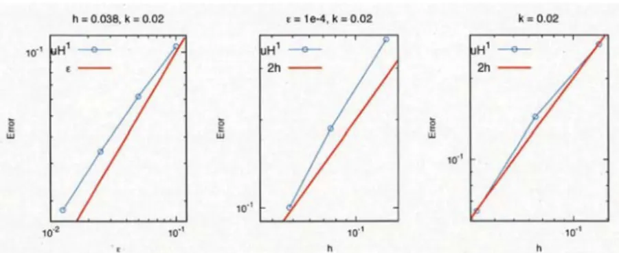
(9) 52. hE0.03\varepsilon, k=0.02 \iota=1\varepsilon-4.\aleph=0.02 k=0.02 10^{-}. t\downarowJ\xi. w\xi. \iotau\xi. t0. t0^{\cdot}. 10^{2}. 10^{1}. 10^{1}. l0'. b. h. Figure 2: (left) T1le error \Vert u_{f}^{11I}-u_{h}^{f1^{\prime 1}}\Vert_{H^{1}( ) } for different pel\rfloor alty p a\cdot anleter \epsilon with fixed lnesh size h=0.038 and \triangle t=0.02 . (nliddle) The error \Vert u_{f}^{1_{1}f}-u_{h}^{1\backslash I}\Vert_{H^{1}(\zeta) } for different lllesh size h witll fixed penalty paranleter \epsilon=10^{-4}al\perp d\triangle t=0.02 . (right) The error \Vert u_{f}^{I}\iota x-u_{h}^{\int 1I}\Vert_{H^{1}(1l)} for different ltlesh size h with \triangle t=0.02 for the. Lagrange lllultipıier approach.. (Step 4). With obtained. (u_{h}^{m.(j)}, p_{h}^{m.(j)}) ,. we calculate. \lambda_{h}^{7r\iota.(j)} ,. which satisfies: for aıl v_{h}\in V_{h()},. c( \tau_{hn}), \lambda_{h}^{rn.(j)})=(f^{m}, v_{h})_{S1}-\frac{1}{\triangle t} (u_{h}^{m.(j)}-u_{h}^{m-1}, v_{h})_{(2}-a_{1}(u_{h}^{m}.(j),mu_{h}(j), v_{h}) -a(u_{h}^{m.(j)}, v_{h})-b(v_{h}, p_{h}^{m.(j)}). (4.9). ,. (Step 5). Increase j by 1 and iterate (Step 2)‐(Step 4) until convergence.. u_{hn}^{\tau n.(j)}\lambda_{h}^{m.(j)}=0 on \Gamma_{out} is satisfied at each iterationl. In fact, at (Step 3), t ]] problenl (4.8) \lambda_{h}^{m.(j)}=0 on the active set A^{m.(j)} . On the other hand, u_{h\uparrow\iota}^{m.(j)}=0 on the inactive set I^{m.(j)} is explicitly inaplenlented. Hence, we have u_{hn}^{m(j)}\lambda_{h}^{m.(j)}=0on1I^{7\gamma\iota.(j)}\cup A^{7\tau L.(j)}= \Gamma_{out}. Tıle conditionl. e. inlplies that. 5 5.1 5.1.1. The numerical experiments The convergence rate The convergence rate of the penalty approach. We investigate. t1_{1}eco ] lvergence. rate of the penalty approach by nunterical experinlent. We siınulate the. flow in donlain \Omega :=\{(x, y) 0<x<3, -1<y<-1, (x-0.4)^{2}+y^{2}>0.4^{2}\} with inflow boundary \Gamma_{\tau n} :=\{(x, y)|x=0\} , the no‐slip boundary \Gamma_{()} :=\{(x, y)|y=\pm 1\} , and the outflow boun dary \Gamma_{out} \{(x, y)|x=3\} . We set the viscosity v=0.01 and the inflow velocity g=2(1+0.3\sin(2\pi t))(1-y^{2}) on \Gamma_{in}. For a very fine mesh T_{f} and tiny penalty paranleter \epsilon_{f} and time‐step size \triangle t , we conlpute the nulnerical :=. solution at. \prime 1^{\rceil}=0.6_{\backslash .}. which is denoted by. (u_{f}^{f1I_{\backslash } .p_{f}^{l\backslash j}) .. We regard. (u_{f^{1} ^{JI},p_{f}^{11I}). as the exact solution and calculate. the error \Vert u_{f^{I} ^{\int_{1} -u_{h}^{AI}\Vert_{H^{1}(\Omega)} , where u_{h}^{M} is the discrete solution with coarser lnesh T or t1_{1}e penalty paralneter \epsilon(\epsilon_{f}<\epsilon\ll 1) First, we fix t1_{1}e mesh T_{f} , and plot the errors for different \epsilon in Figure 5.1.1 (left), which i_{1]} dicates the .. convergence of order O(\epsilon) . Next, for fixed pe1lalty paraAneter C we con pute the error for different nlesh size h (see Figure 5.1.1 (llliddle)), which shows the convergence of order O(h) .. For the Lagrange ntultiplier approach, we investigate the convergence order depending on lnesh size h with a fixed tinle‐step size \triangle t . The error is plotted in Figure 5.ı. 1 (right), which also shows the O(h) ‐convergence..

(10) 53. 0. 0.. 0.. \delta\not\ino\Phi0(. u^{o}\existgbule. 0 0 0. t. t. Figure 3: The drag. 0. al. d. lift forces ior \nu=9.76\cross 10^{-1)}\ulcorner. 0. (. 0.. 0.. 0.. \per og\infty. ]. 88. (. u_{-}z\supset0\prec. \Xi 0. 0.. 0. 0. \{. 0. \triangleleft. 0. 5. 10. \dagger 5. 20. 2S. SO. 0. 5. 10. t. 20. \approx. $. 1. Figure 4: The drag and lift forces for 5.2. 15. \ulcorner. \nu=4.88\cross 10^{-\backslash } ). The numerical simulations. To validate the suitability of applying the Signorini boundary condition for real‐world fluid silnulation, we conlpare the simulation results to the experinlental data. We silnulate the flow in dolnain \Omega :=\{(x, y) 0<x<2.5L. -L<y<-L, (x-0.5)^{2}+y^{2}>r^{2}\} and tilne interval (0, (1^{\gamma}) , where \ulcorner 1^{\rceil}=30, r=0.1, L=1, \Gamma_{in} :=\{(x, y)|x=0\} , the no‐slip boundary \Gamma_{()} :=\{(x, y)|y=\pm L\} , and the outflow boundary \Gamma_{ovt} :=\{(x, y)|x=2.5L\} . The i_{l1} flow velocity is given by g=L^{2}-y^{2} on \Gamma_{in} . We conlpute the drag force D_{f} and tıle lift force L_{f} on the circle boundary C_{1} :=\{(x, y)|(x-0.5)^{2}+y^{2}=r^{2}\} :. D_{f}:=- \int_{C_{1} \sigma(u,p)n\cdot dds, L_{f}:=\int_{C_{1} \sigma(u, p) n\cdot lds, where d=(1,0)^{T} and l=(0,1)^{T} We plot two profiles of the drag and lift forces in Figure 5.2 and Figure 5.2 for \nu=9.76\cross 10^{-\ulcorner} and \nu=4.88\cross 10^{-(}\ulcorner respectively. The average of drag and lift forces for various Reynolds. nunrber \propto Re=v-{\imath} are plotted in Figure 5.2, which sonlehow corresponds to. t1_{1}e. experinlental data [8] for. \nu\geq 10^{-}. References [1] Y. Bazilevs, J. R. Hol] eall, T. J. R. Hughes, R.. D. Moser, and Y. Zl] ang. Patient‐specific isogeo] netric fluid‐structure interaction analysis of thoracicaortic blood flow due to i_{111} plant ationof t1) e Jarvik2000 left ventricular assist device. Comput. Methods Appl. Mech. Eng., 198:3534-3550_{\backslash }. 2009..

(11) 54. 0^{o} 1 1. {\rm Re}. {\rm Re}. Figure 5: The average drag and ıift forces for different Re =\nu^{-\rfloor}. [2] F. Boyer and P. Fabrie. Outflow boundary conditions for the incompressibıe non‐homogeneous Navier‐ Stokes equations. Discrete and Continuous Dynamical Systems‐Serves B. American Institute of Mathe‐ matical Sciences, 7:219−250, 2007.. [3] C.‐H. Bruneau and P. Fabrie. Effective downstreanl boundary CO1] ditions for inconlpressible Navier‐ Stokes equations. Int. J. Numer. Methods Fluids, 19:693−705, 1994.. [4] C.‐H. Bruneau and P. Fabrie. New efficient boundary conditions for. i_{1]Con1} pressible. Navier‐Stokes equa‐. tions: a welı‐posedness result. Math. Model. Numer. Anal., 30:815−840, 1996.. [5] S. Dong. A convective‐like energy‐stable open boundary condition for silnulations of inconlpressibıe flows. J. Comput. Phys., 302:300−328, 2015.. [6] S. Dong and J. Shen. A pressure‐correction schelne for generalized fornl of energy‐stabıe open boundary conditions for inconnpressible flows. J. Comput. Phys., 29ı:254‐278, 2015.. [7] N. Kikuchi aıld J. T. Oden. Contact Problems in Elasticity. SIAM, ı988. [8] C. Norberg. Fluctuating ıift on a circular cyıinder: review and new lneasurenlen]ts. Journal of Fluids and Structures, 17:57−96, 2003.. [9] N. Saito, Y. Sugitani, anld G. Zhou. Energy inequal_{i}t_{i}es and outflow boundary conditions for the Navier‐ Stokes equations, chapter Advances in conlputational fluid‐structure i_{lJ}teracti_{o1)}al\rfloor d flow New nlethods and challenging computations, pages 307‐317. Birkhauser, 2016.. si_{1} ) \rflo r ulation:. [10] N. Saito, Y. Sugitani, and G. Zhou. Unilateraı problem for the Stokes equations: the well‐posedness and finite elentent approxinlation. Appl. Numer. Math., 105:124−147, 2016.. [11] G. Zhou and N. Saito. The Navier‐Stokes equations under a unilateral boulıdary condition of Signorini’s type. Journal of A4athematlcal Fluid Mechanics, 18:481-510_{\grave{t}} 2016..

(12)