Mach reflection of a solitary wave: seeking the four-fold amplification (Workshop on Nonlinear Water Waves)

全文

(1)135. Mach reflection of a solitary wave: seeking the four‐fold amplification Harry Yeh and Jeffrey Knowlesl. lSchool of Civil and Construction Engineering, Oregon State University, Corvallis, OR 97331, USA September 18, 2018 Abstract. The laboratory and numerical experiments are presented for the Mach reflection of an obliquely incident solitary wave at a vertical wall. The numerical model is based on the pseudo‐ spectral method for the full Euler formulation: the model is an extension of that used by Tanaka. (1993). With the aid of a laser sheet in the laboratory, the wave profiles are measured optically in sub‐millimeter precision. Discrepancies reported in previous works are now substantially improved, partly because of the higher‐order KP theory but also in part of advancements in computational power and laboratory instrumentation. A maximum amplification of 3.91 is. achieved along the wall, nearly realizing the four‐fold prediction by Miles (1977b) .. 1. Background. More than 60 years ago, Perroud (1957) experimentally demonstrated the reflection of a solitary wave with oblique incidence along a vertical wall. The reflection pattern observed in the wave tank resembled the formation of a Mach stem: a well‐known phenomenon for compressible shock waves. (e.g. von Neumann (1943); Courant & Friedrichs (1976)). When a shock wave impinges on a wall with a small incident angle, a three‐wave configuration emerges near the wall; 1) the incident wave, 2) reflected shock fronts, and 3) the continually growing (Mach stem” which forms perpendicular to the wall. The reflected shock front branches off from the incident shock away from the wall at the outer edge of the Mach stem. Figure 1 depicts the formation of the Mach reflection of a solitary wave, in which the reflected wave angle \psi_{r} is greater than the incident wave angle \psi_{i} . Even though the governing equations for compressible fluids are similar to the shallow‐water wave equations, Perroud’s experimental work in 1957 which demonstrates the realization of the Mach reflection for solitary waves in the laboratory environment is still quite remarkable.. Inspired by Perroud’s laboratory results, Miles (1977a,b) analyzed obliquely incident solitary waves onto the reflective boundary (i.e. the vertical wall), based on the assumption of shallow‐but‐ finite water depth and small‐but‐finite wave amplitude. Miles found that there exists an angle \psi_{c} such that if the incidence angle \psi_{i} is larger than \psi_{C} , the reflected wave behind the incident wave has the same angle \psi_{i} with a phase shift at the intersection, i.e. regular reflection. If the angle is smaller than \psi_{c} , then the Mach stem appears and its crest length continuously grows as illustrated in figure 1. The incident wave, the reflected wave, and the Mach stem interact and form a resonant.

(2) 136. Figure 1: Mach reflection: \psi_{i} , incident wave angle; \psi_{r} , reflected wave angle. triad. Miles’s prediction for the maximum wave amplification \alpha_{w} ‐ the ratio of the wave amplitude a_{w} at the wall to the incident wave amplitude a_{i}, \alpha_{w}=a_{w}/a_{i} ‐ is expressed as:. \alpha_{w}=\{ begin{ar ay}{l} (1+k)^{2}, fork<1, \frac{4}{1+\sqrt{1-k2}, fork>1, \end{ar ay} where. k. (1). is the parameter defined by:. k= \frac{\psi_{i} {\sqrt{3a_{i} , in which Miles found that \psi_{C}=\sqrt{3a_{i}} (or. k=1.0 ). (2). under the assumption of a small angle. Note that. Miles assumed that \sin\psi_{i}\approx\psi_{i} , which turns out to be the key assumption that causes discrepancy between the predictions and the experiments. Miles derived formula (1) under the assumption of small incidence angle \psi_{i} , which is referred to as a strong interaction. In the case of large \psi_{i} (he assumed \sin^{2}\psi_{i}\gg a_{i} ), Miles obtained the following formula for the maximum amplification:. \alpha_{w}=2+a_{i}(\frac{3}{2s\dot{ \imath} n^{2}\psi_{i} -3+2\sin^{2}\psi_{i} ) .. (3). It is significant to note that Miles’s theory predicts the maximum possible amplification to be four fold: \alpha_{w}=a_{w}/a_{i}=4 when k=\psi_{i}/\sqrt{3a_{i}}=1.0 . Here, the parameter a_{w} is the normalized amplitude at the wall, and a_{i} is the incident wave amplitude normalized by the still water depth h_{0} . Hereinafter the length is normalized by h_{0} and time is normalized by \sqrt{g}/h_{0} where g is the gravitational acceleration. Our intuition tells us that the amplification should be two \alpha_{w}=a_{w}/a_{i}=2 when the incident wave collides perpendicularly with the wall, while the wave propagating parallel to the wall yields no amplification \alpha_{w}=a_{w}/a_{i}=1 . Therefore, this four‐fold amplification is surprising and important.. Because of Miles’s remarkable prediction of four fold maximum amplification, Melville (1980) attempted to validate Miles’s theory in the laboratory tank but only attained an amplification of less than 2.0 at the wall: his attempt completely failed. Almost at the same time as Melville’s. laboratory experiments, Funakoshi (1980) conducted numerical experiments to verify Miles’s theo‐ retical predictions, but only achieved a maximum amplification of \alpha_{w}\approx 3.45 . It is not surprising that Funakoshi’s numerical results are in better agreement with the theory because the governing equations are the same as Miles’s limits. In other words, Funakoshi’s work can be considered as a.

(3) 137. \alpha_{w}. k. Figure 2: Amplification predicted by Funakoshi (1980) Miles (1977a,b) ’s theoretical prediction (1).. \cross. and Tanaka (1993). \triangle .. Solid line represents. verification of Miles’s prediction, rather than a ‘validation’. Nonetheless, Funakoshi could not nu‐ merically demonstrate the critical amplification of \alpha_{w}=a_{w}/a_{i}=4 . Note that Funakoshi presented the results for a_{i}=0.05 with \psi_{i}=2.25^{\circ}\sim 30^{\circ} , and commented that it takes a very long time to. achieve the stationary Mach‐reflection pattern. Unlike Funakoshi (1980) whose numerical model is the same order of approximation as the theory by Miles (1977a,b) , the numerical experiments by. Tanaka (1993) were based on a higher‐order pseudo‐spectral method to solve the full Euler formula‐ tion. This higher‐order model allowed him to study conditions less restricted by \psi_{i} and. a_{i} .. However,. Tanaka (1993) achieved a maximum amplification of \alpha_{w}=2.897 at k=0.644. Li et al. (2011) revisited the problem, performing laboratory experiments with a wave basin (7.3 m long and 3.6 m wide with a water depth of 6.0 cm). They found that discrepancies between the previous laboratory results (Perroud (1957); Melville (1980)) and Miles’s prediction (1) are attributed partly to the insufficient propagation distance in the laboratory experiments so that the asymptotic state could not have been reached. Figure 3 shows the measured data with Miles’s parameter k . The result exhibits a peak in amplification at the Miles parameter k=0.753 . The measured maximum amplification factor is \alpha_{w}=2.92 which is less than Miles’s four‐fold prediction, but is substantially more than what is predicted by linear superposition. Miles (1977b) introduced the interaction parameter k=\psi_{i}/\sqrt{3a_{i}} in order to predict wave am‐. plification. Based on the KP theory, (Kadomtsev & Petviashvili (1970); Li et al. (2011)) proposed the following modification:. k= \frac{\tan\psi_{i} {\sqrt{3a_{i} \cos\psi_{\dot{i} .. (4). The primary motivation behind (4) is to remedy the KP soliton paradox which states that the breadth of a soliton depends on \psi_{i} . The incident waveform corresponding to (4) is however no longer an exact solution to the KP equation. To achieve a consistent theory, a normal form of the. KP equation with higher order corrections was derived by Kodama & Yeh (2016) resulting in the following. k. value:. k= \frac{\sqrt{1+\sqrt{1+5a_{i} \tan\psi_{i} {\sqrt{6a_{i} \cos\psi_{i} together with the newly defined KP amplification:. ,. (5).

(4) 138. \alpha_{w}. k. Figure 3: Experimental results of the amplification factor. circle circle. 0 e. \alpha_{w}. show the results of Perroud (1957), the open square is the data by Li et al. (2011).. versus Miles’s parameter \square. k.. The open. show Melville (1980), and the solid. \hat{\lpha}=\{begin{ar y}{l \frac{\lpha_{w}(1+\sqrt{1+5a_{i}) (1+\sqrt{1+5\alph_{w}a_{i})\cos^{2} \psi_{}, fork<1, \alph_{w}, fork>1. \end{ar y}. (6). With the use of (5) and (6) a substantial improvement is made in predictability. From here on out k will refer to equation (5). The numerical and laboratory results are now evaluated with the new formulae (5) and (6) based on the higher‐order KP theory and the results are shown in figure 4. Laboratory data by. Perroud (1957) and Melville (1980) are not presented here because the propagation distance in their experiments was too short to achieve the asymptotic state. Since Funakoshi (1980) ’s numerical simulations are conducted with small incident waves (a_{i}= 0.05) , his results match the KP predictions very well. Tanaka (1993) ’s results also match the theory;. the higher‐order correction substantially shifts his numerical data to the positive k value. Note that Tanaka’s numerical experiments are made with the relatively large value of a_{i}=0.3 , and a large value of the incidence angle \psi_{i} . The agreement of Tanaka’s results with the KP theory is not as good as Funakoshi’s, especially not for the data near k=1 . This is because the KP theory, even higher‐order, still assumes that the value of a_{i} and \tan\psi_{i} are small. Figure 4 also shows that the higher‐order KP theory results in substantial improvement in agreement of the laboratory data with the theory.. To obtain the maximum amplification near. k\approx 1 ,. Tanaka (1993) used an incident wave amplitude. of a_{0}=0.3 in his numerical experiments, and Li et al. (2011) ’s laboratory experiments used an amplitude of a_{0}=0.277 . The resulting amplifications for both numerical and laboratory experiments are \hat{\alpha}\approx 3 . Even Funakoshi (1980) ’s numerical simulation that follows Miles (1977a,b) ’s analytical model presents a maximum amplification of \hat{\alpha}=3.42 at k=0.87 . Because the wave amplitude along the wall is close to unity (\neq \mathcal{O}(\varepsilon)) , the assumption of weak nonlinearity is clearly violated. Here we attempt to compute numerically the Mach reflection to achieve the four‐fold amplifica‐ tion. The full Euler model is used so that the outcome can be considered as a validation of Miles’s.

(5) 139. \hat{\alpha}. k. Figure 4: Numerical and experimental results of the KP amplification factor \hat{\alpha}(6) versus the new. higher‐order KP parameter (5). The crosses \cross show the numerical results by Funakoshi (1980), the hollow triangles \triangle show the numerical results by Tanaka (1993), and the solid circles are the laboratory data by Li et al. (2011). e. analytical prediction. We follow the same approach as Tanaka (1993), but use a much finer compu‐ tational resolution and much longer simulations, which is possible due to computer advancements that have taken place since Tanaka’s work in 1993.. 2. Numerical methodology. The Zakharov‐Craig‐Sulem formulation (Craig & Sulem (1993); Zakharov (196S) ) of the full water‐ wave equations is solved numerically. A higher‐order pseudo‐spectral method developed by Dom‐. mermuth & Yue (1987) is used, and this numerical scheme is practically the same as that used by Tanaka (1993). The initial conditions for the velocity potential at the water surface \Phi^{S} and the surface displacement. \eta. are prescribed by the higher‐order solitary wave solution given by Grimshaw. (1971):. \eta=a_{i}S^{2}-\frac{3}{4}a_{\dot{i} ^{2}(S^{2}-S^{4})+a_{i}^{3}(\frac{5}{8} S^{2}-\frac{151}{80}S^{4}+\frac{101}{80}S^{6}). ,. \Phi^{S}=2\sqrt{\frac{a_{i} {3} \{T+a_{i}[\frac{5}{24}T-\frac{1}{3}S^{2}T+ \frac{3}{4}(1+\eta)^{2}S^{2}T]+a_{i}^{2}[-\frac{1257}{3200}T+\frac{9}{200}S^{2}T +\frac{6}{25}S^{4}T+ (1+ \eta)^{2}(-\frac{9}{32}S^{2}T-\frac{3}{2}S^{4}T)+(1+\eta)^{4}(- \frac{3} {16}S^{2}T-\frac{3}{2}S^{4}T)]\}. In (7),. S. and. T. (7). are S=. sech \kappa(x-x_{0}), T=\tanh\kappa(x-x_{0}) , inwhich. \kap a=\sqrt{\frac{3}{4}a_{i} (1-\frac{5}{8}a_{i}+\frac{71}{128}a_{i}^{2}) .. (8).

(6) 140. (a).. (b). \eta 0.. -20. ‐ 10. 0. 10. 20. ‐ 30. ‐IS. x. 0. 15. 30. x. Figure 5: (a): Overlay of solitary wave for a_{i}=0.1, \psi_{i}=0^{\circ} . (b): Overlay of solitary wave for a_{i}=0.03 and \psi_{i}=15^{\circ} where the boundary condition is treated to eliminate wave deffraction. In both cases t=313.2 solid line, t=3132 dashed line, t=6264 circles.. This solution is correct up to 3^{rd} order, so the perturbation expansion is also truncated at the. third term. At the offshore boundary (away from the reflective wall), the wave crest is artificially extended to circumvent the artificial effects of wave diffraction. On account of the initial conditions. being a‐periodic, the domain is extended periodically in the horizontal directions to accommodate for the Fourier basis functions. It takes a very large domain to run the simulation to reach the asymptotic state, causing the calculation to be quite formidable. A computer with a CPU of 3.40 GHz was used to simulate a number of cases for various combinations of a_{i} and \psi_{i} . This allows us to use a large domain where the number of nodes in the x and y direction are N_{x}=2^{13} and N_{y}=2^{10},. respectively. Note that Tanaka (1993) used N_{x}=128 and N_{y}=512 . The spatial resolution in the. x and y direction is taken to be dx=(4\kappa\sin\psi_{i})^{-1} and dy=(4\kappa\cos\psi_{i})^{-1} , respectively. The time step used ranged from 0.157 to 0.196 which insured that the Courant number is always less than one.. The numerical algorithm is verified by checking conservation of volume and energy for a solitary wave where a_{i}=0.1 and \psi_{i}=0^{\circ} . Figure 5a shows that the amplitude of the solitary wave does not change, indicating that energy is conserved. We found that the greatest error for conservation of volume is -0.0022 % which is likely caused by the initial condition given by the 3^{rd} order solution, which is not exact.. In certain trials (when \psi=10^{\circ} and 15^{0} for values of k close to unity), it is necessary to perform a translation on \Phi^{S} and \eta due to the long propagation time. This translation is performed before the leading crest reaches the end of the domain. The translation is given by \Phi_{new}^{S}(x, y, t)=. \Phi^{S}(x-X_{new}, y, t). and. \eta_{new}(x, y, t)=\eta(x-X_{new}, y, t). where. \Phi_{new}^{S}. and \eta_{new} are the translated. values of the free‐surface velocity potential and surface displacement, respectively. This process is repeated in a cyclic manner until the simulation is terminated. The leading crest is also extended in order to prevent the effects of diffraction along the offshore boundary from the wall. An overlay is presented in figure 5b for the case a_{i}=0.03, \psi_{i}=15^{\circ} . The overlays are calculated by taking a cross section perpendicular to the crest in a region where the extension algorithm is being applied. The phase speed is also checked for this case and the maximum value of relative error between the. measured phase speed and theoretical higher‐order phase speed (Grimshaw 1971) is −0.009%.. 3. Results. Three different incident‐wave angles were examined ( \psi_{i}=10^{\circ}, 15^{o} , and 26^{\circ} ) for a range of interaction parameters (0.5\leq k\leq 1.31) . We also revisited the work of Tanaka (1993) by extending the.

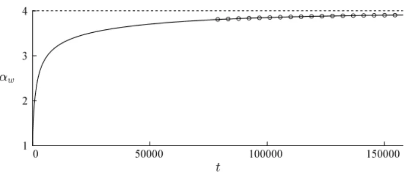
(7) 141 141. \alpha_{w}. 0. 50000. 100000. 150000. t. Figure 6: Evolution of amplitude for the case a_{i}=0.0108, k=1.0, \psi_{i}=10^{\circ} . Solid line is amplification at wall. Circles are the fit polynomial used to calcute that the slope at t=157860 is 3.00\cross 10^{-9}.. simulation times for a_{i}=0.3 with \psi_{i}=30^{\circ}, 35^{\circ} , and 40^{\circ} . Figure 6 shows how small the growth rate had to be before terminating the simulation. The wave amplification is plotted against the. interaction parameter k(5) in figure 7, where the KP amplification \psi_{i}=10^{\circ} and a_{i}=0.0108(k=1.0) .. \hat{\alpha}. is given by (6). An amplification. of \hat{\alpha}=3.91 is achieved when. We also examine the length of the stem wave formation for three different cases: (\psi_{i}=26^{\circ}, k= 0.90), (\psi_{i}=10^{\circ}, k=1.0) , and (\psi_{i}=15^{\circ}, k=1.01) . In the first case, the Mach stem length is. conitnually growing even after the amplitude at the wall has reached an asymptotic state. For the latter two cases, the stem length has stopped growing by the time the amplitude at the wall has reached an asymptotic state. This observation of the numerical experiments is consistent with the. theoretical prediction made by Miles (1977a,b) and more explicitly by Kodama & Yeh (2016). The results by Funakoshi (1980) for a_{i}=0.05 are also presented in figure 7a . The good agreement seen in Funakoshi’s results comes from the fact that he solved equations that are on the same order of approximation as Miles’s theory. Comparison of the solid and hollow triangle symbols in figure 7b demonstrates a clear improvement of the present data over Tanaka’s, particularly for the case of. 30^{\circ}(k=0.789) When. and. 35^{\circ}(k=1.024) .. k<1 a three‐wave resonant interaction occurs. On the other hand when. k>1 the KP. solution is described as a simple reflection accompanied by a phase shift. When k=1 there is a weak discontinuity‐type singularity and the interaction is no longer clearly defined. After this point k=1^{+} the amplification begins to drop off very sharply which appears to be in agreement with the numerical results.. After computing the amplification at various k values, we see that there is a dependency on \psi_{i} near k\approx 1 as shown in figure 7c and the data no longer agree well with the theoretical curve. These results show that \hat{\alpha} shifts down and to the right as \psi_{i} increases. The open circle and open triangle. overlap nicely for k=0.8 . The angles used in these two different simulations were similar (open triangle: \psi_{i}=30^{\circ} , open circle: \psi_{i}=26^{\circ} ). However, the nonlinearities are considerably different (open triangle: a_{i}=0.3 , open circle: a_{i}=0.1 ), indicating that the incident wave angle appears to have more of an impact on the amplification than the nonlinearity. At k=0.8 we see that the amplification appears to increase monotonically as the angle of incidence is decreased..

(8) 142 (a) 4 3. \hat{\alpha} 2. 1. K.. (b). \sim. \hat{\alpha}. 0.0. 10. ZO. 30. k. 0.7. 0.8. 09. 1.0. 1. 1. 1.2. k. Figure 7: Amplification for several higher‐order interaction parameters. Solid line is theoretical curve, A= Tanaka original, \triangle= Tanaka new, \cross= Funakoshi, O=10^{\circ} , square =15^{\circ}, 0=26^{\circ}. (a). All the data; (b) comparison of Tanaka’s data (c) closeup view of data near. 4. k=1.0.. Conclusions. The oblique incidence of solitary waves at a vertical wall is studied. A higher‐order pseudo‐spectral method is implemented in order to simulate experiments for \psi_{i}=10^{\circ}, 15^{\circ} , and 26^{\circ} for various interaction parameters (0.5\leq k\leq 1.31) . We also re‐computed the cases presented by Tanaka. (1993), resulting in improvement after substantially extending the simulation time.. All results. are then compared with the theoretical prediction of Miles (1977b) after converting the results to. the higher order KP theory given by Kodama & Yeh (2016). The greatest amplification achieved. is \hat{\alpha}=3.91 when a_{i}=0.0108, \psi_{i}=10^{\circ} , almost realizing the four‐fold prediction. It appears that the amplification is sensitive to the angle of incidence when k is near unity. By performing these simulations with the full water‐wave model, we have provided results which contribute to the quantitative validity of Mile’s theory, at last.. References Courant, R. & Friedrichs, K. (1976), ‘Supersonic flow and shock waves (interscience, new york, 1948)’, Google Scholar p. 141. Craig, W. & Sulem, C. (1993), ‘Numerical simulation of gravity waves’, Journal of Computational Physics 108(1), 73‐83.. Dommermuth, D. & Yue, D. (1987), ‘A high‐order spectral method for the study of nonlinear gravity waves’, Journal of Fluid Mechanics 184, 267‐288.. Funakoshi, M. (1980), ‘Reflection of obliquely incident solitary waves’, Journal of the Physical Society of Japan 49(6), 2371‐2379..

(9) 143 Grimshaw, R. (1971), ‘The solitary wave in water of variable depth. part 2’, Journal of Fluid Me‐ chanics 46(3), 611‐622. Kadomtsev, B. B. & Petviashvili, V. I. (1970), On the stability of solitary waves in weakly dispersing media, in ‘Sov. Phys. Dokl’, Vol. 15, pp. 539‐541.. Kodama, Y. & Yeh, H. (2016), ‘The kp theory and mach reflection’, Journal of Fluid Mechanics 800, 766‐786.. Li, W., Yeh, H. & Kodama, Y. (2011), ‘On the mach reflection of a solitary wave: revisited’, Journal of fluid mechanics 672, 326‐357.. Melville, W. (1980), ‘On the mach reflexion of a solitary wave’, Journal of Fluid Mechanics 98(2), 285‐297. Miles, J. (1977a) , ‘Obliquely interacting solitary waves’, Journal of Fluid Mechanics 79(1), 157‐169. Miles, J. (1977b) , ‘Resonantly interacting solitary waves’, Journal of Fluid Mechanics 79(1), 171‐ 179.. Perroud, P. (1957), The solitary wave reflection along a straight vertical wall at oblique incidence, Technical report, U.C. Berkeley, Calif.. Tanaka, M. (1993), ‘Mach reflection of a large‐amplitude solitary wave’, Journal of fluid mechanics 248, 637‐661.. von Neumann, J. (1943), ‘Oblique reflection of shocks’, John von Neumann Collected Works 6,. 23S-. 299.. Zakharov, V. (1968), ‘Stability of periodic waves of finite amplitude on the surface of a deep fluid’, Journal of Applied Mechanics and Technical Physics 9(2), 190‐194..

(10)