Numerical analysis of a tag model in circle (Mathematical models and dynamics of functional equations)

(1)

Numerical

analysis

of

a

tag model

in

circle

Makoto IIMA(飯間信)” and Keita SUZUKI(鈴木啓太)

Nonlinear Studies and Computation,

Research Institute

_for

Electronic Science,

Hokkaido University, Sapporo 060-0812, Japan \mbox{\boldmath $\theta$}b海道大学電子科学研究所) Department

_of

Mathematics, Hokkaido University, Sapporo 060-0810, Japan \mbox{\boldmath $\theta$}b海道大学大学院理学研究科)

We analyzed asimplest tagmodelonacircle. This problemconsistsofoneperson

to chase and one to elude, and the output force to move is a function of the

rela-iive position. The effect oftime delay from collecting the information to output is

considered. This model shows vai’ious motion including chaotic one, which can not

beobservedwithout thetime delay. Whenreplacingthe delay term toadistributed

one, some chaotic motionis stabilized.

I. INTRODUCTION Time delay appears in

many

kinds of

dy-namical system such

as

demography

(mat-Chasing is ubiquitous

around

us.

Tag is uration time), epidemic (incubation time),

atypicalchildren’s gamein which

one

chases control systems(transmission

of feedback

sig-the rest. In

a

ball game such

soccer

of bas- $\mathrm{n}\mathrm{a}\mathrm{l}$), economy (time lag from the

measure-ketball,

a

person possessing ball

are

chased ment to the

announce

of the economic

in-by the defense. The dynamics of the per- dicators ), optics (feedback signal of light) son to chase(“chaser”) and the person to [1, 3, 4]. It is known that time delay

desta-elude(“eluder” ) is not trivial: the chaser col- bilize

a

fixed point andinvokes complex

phe-lects the information of the eluder (position, nomena suchas chaos.

velocity, etc.), process the information, and _In _this _paper,

_we

$\mathrm{m}$ ake a simplest tag

determine the amount and the direction of _{model to understand the} _chasing _dynamics.

the output force, and vice

versa.

In general, _Our

aim here is to know how the time

de-processinginformation costs

a

finitetime. In _{lay changes the} _result

of chasing without de this study,

we

focus

on

the effect of the time _{lay. In particular,}

_we

_assume

_{that the chaser}

delayto process the information. _{and the eluder}_{have similar moving principle.}

Timedelay in adynamical system iscom- _Furthermore,

_we

_{choose the maximum}_{of the}

mon

in nature. A_{typical example is the mat- output} _function

_{as a}

_parameter _of _the

abil-uration time of man to reproduce the next $\mathrm{i}\mathrm{t}\mathrm{y}$to

move.

The difference of the parameter

generation. It takes a finite time that

a

_{dis- between}_the _{chaser and the}_{eluder is}

_an

indi-turbance of birth rate is reflected in

a

next _cator _to _predict _{the result} _of _the _{chase. An}

generation. When this effect is taken in

a

_{naive expectation is that the sign of the}

in-population model, it contains delay term[l]. _dicator _is

_a

_unique _factor _to _{determine the} result. Onthe other hand, time delay

causes

$\overline{*\mathrm{E}\mathrm{l}\mathrm{e}\mathrm{c}\mathrm{t}\mathrm{r}\mathrm{o}}$

nic address: makotoflaurora.es.hokudai. _to _{destabilize the fixed} point. These two

ele-$\mathrm{a}\mathrm{c}$.jp; $\mathrm{b}^{1}\mathrm{R}\mathrm{L}$: $\mathrm{h}\mathrm{t}\mathrm{t}\mathrm{p}://\mathrm{a}\mathrm{u}\mathrm{r}\mathrm{o}\mathrm{r}\mathrm{a}$.es.hokudai.$\mathrm{a}\mathrm{c}.\mathrm{j}\mathrm{p}/$ ments may be ill conflict,

so

the behavior of

(2)

In sec.II, we show tlle detail of the model This equation

can

be rewritten intermsof Sec. III is devoted to show the numerical $z(t)$ only as follows:

result of the model. Linear stability theory is applied to this model in $\mathrm{s}\mathrm{e}\mathrm{c}$. $\mathrm{I}\mathrm{V}$. $z.$

.

$(t)+CF(z(t-\tau))+K\dot{z}(t|)=0$_, (4)

where$C=A-B$istheparameterto

measure

$\mathrm{I}\mathrm{I}$

.

MODEL _the _maximum _of _{the output} _{force $(C>0$}

means

$X$(chaser)haslarger outputforcethan

Weconsider tag model ina unitcircle with $Y$(eluder)$)$

.

one

chaser(X) and

one

eluder(} ). Each posi- _{The definition of the} _{capture is}_{as follows:} tionof$X$ and $\mathrm{Y}$,

$x$ and$y$, is measuredbythe in this simple situation, a naive definition of

arc

length from an origin. _{The dynamics of the catch, such}

_as

_{the state} $|\mathrm{z}(\mathrm{t})|<\exists\epsilon_{\}}$ for$\exists t$

$X$ and $Y$ is given by the following equations:

can

not lead

us

to interesting results. Thus

we

define the catch

as

thestate$z(t)arrow 0(\mathrm{a}1\mathrm{s}\mathrm{o}$

$x(t)+A$$F$(z$(t-\mathcal{T})$) $+Ki(t)=0$ , (1) $\dot{z}(t)arrow$? 0)

as

$tarrow\infty$

.

This definition

means

that catching $\mathrm{Y}$ requires not only the rela-$y..(t)+BF(z(t-\tau))+K\dot{y}(t)=0$_, _{(2) tive position} _but _{the relative} _velocity_should

$z(t)=y(t)-x(t)$ (3) be

zero. A

simplest example to satisfy this

conditionistag

among

two agile persons.

An

where $\dot{x}$

means

time derivative of

$x$, $A$,$B$,$K$

instant time of coincidence is insufficient to

are

positive constants. The output force is _catch _{the eluder: he}

_can

_{slip through} _from

determinedby $F(z)$

as

a

functionof the rela- the _chaser’s

_arms.

tive positionof$X$ and$Y$, $z$ $=z(t)$. Torealize

In this paper,

we

report the

case

$F(x)=$

the situation in tag, $F(z)$ should be positive _$\sin(x)$_, _{while the} _case _{of the} _other _function

when $0<z$ $<\pi$, negative when yr _$<z$ $<2\pi.$

such as bilinear function$($ $F(x)=x(|x|<$

$\mathrm{I}’\mathrm{h}\mathrm{e}$ output-force function

$F(z)$ is assumed _$\pi/2$_);_{$\pi-x(\pi/2<x<3\pi/2))$} _and

rectangu-odd by the requirement ofthe symmetry un- $\mathrm{l}\mathrm{a}\mathrm{r}$ function(F(x)=l $(0<x<\pi);-1(\pi<$

der space inversion, and it is also assumed $x<2\pi$₎₎ _is _{also studied in ref. [5].} $2\pi$-periodic function because ofthe

period-When$\tau=0,$ the equation (4) corresponds

icityof space. Here

we

assume

_{finite process- to a} _{dumped simple pendulum. In} _{this case,}

ingtime $\mathrm{r}$ from the input

of the information the behavior is simple. Equilibrium points

to

output the force. In this model, the

_{in- are}

$z(t)$ $=0$ and $z(t)=\pi$. If

$C>0$

formation is the relative position of $X$ and

$z(t)=0$ is stable and $z(t)=\pi$ _is

unsta-Y. $\mathrm{b}\mathrm{l}\mathrm{e}$, and if $C<0,$ vice

versa.

In terms of

the tag model, these result is trivial. The

case $C>0(A>B)$ means

the chaser’s

abil-ity to acceleration is larger that the eluder. Thus it isreasonable that the stable equilib-rium point is $z(t)=\dot{z}(t)=0,$ which

means

thestateof the catch. Onthe other hand, the

case $C<0(A<B)$

means

the eluder’sability to acceleration is larger thatthechaser. Thus

the eluder will not be caught by the chaser.

Stable

equilibrium point, $z(t)=\pi,:(t)$ $=0,$

means

thatthe relative position is not

zero.

FIG. 1: Schematicpictureof the tag model. $X$ _In _the _next _section,

we

_{study this model}

and$\mathrm{Y}$movein theunitcircle. _$X$chases$\mathrm{Y}$,while

rirunerically in the

case

of $\tau>0.$ Because$\mathrm{e}$ $\mathrm{Y}$ eludes from X.

(3)

$\mathrm{r}\mathrm{t}$, so that time delay

$\tau$ is unit tiIne. Under

this transformation, we have

$z(t)+cF\{z\{t-1$))$+\mathrm{k}\mathrm{z}(\mathrm{t})=0$, (5)

$c=C\tau^{2}$ _. (6)

$k=K\tau$ (7)

We analyze this equation hereafter.

仮

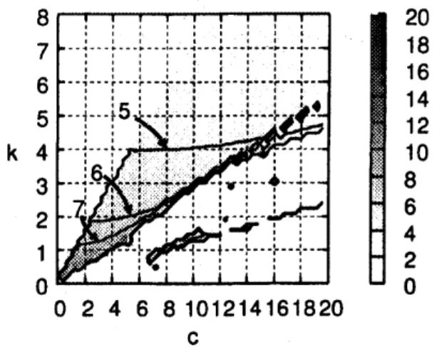
._FIG._2: _Phase_diagram_{of the}_{tag model. For any}

set of$(c, k)$, phase is automatically analyzed

us

ing $\mathrm{z}(\mathrm{t})$, and is characterizedby phase number.

III. NUMERICAL RESULT _In _the_cases _{of (I) and} _(IV), _{phase number} _is _0.

andinthe

cases

of(II) and(III), phase number

Eq.(5) is integrated numerically by the is period number ifit is smaller than 3. When first-Order Euler method with time step$At=$ period number is larger than 3, phase number 0.005. The initial condition is chosen

ran-

is 3. Boundary betweenthe region where phase

domly. Because eq.(5) is invariant under the number is zero and

nonzero

is shown.

transformation

$carrow-c$,$zarrow\pi-z,$

we

only

calculate the

case

$c>0.$ _Parameters $c$ and Wehave

one

stable steady solution $z(t)=$

$k$ is changed in the range

$0<c<20$

and

0

in the region

Co. This

area

is described

$0<k<8.$ by $k>0.8c$ approximately, In this region,

the dump term $ki(t)$ surpasses the

output-force

term

$cF(z(t-1))$

.

Eqs. (6) and (7)

shows

that another interpretation

for

this

phase diagram.

For

example,

the

behavior

of eq. (4) with

a

set of $(C, K, \tau)$ is

equiva-lent to the behavior of eq. (5) with

a

set of

A. Phase Diagram _{$(c, k)=(C\tau^{2}, K\tau)$}

_.

_Therefore, _if

_one

_{want to}

consider how the behavior of eq. (4) varies

We analyzed the time variation oftherela- under the del.ay time $\tau$ with fixed $C$ and $K$,

tive position, $z(t)$, after transitiontime. The the change of thebehavior is shownalongthe

datais classified intothe following fourcate parabola $k= \frac{K}{\sqrt{c}}\sqrt{c}$in fig. 2.

gories (fig.2): (I) convergence($z(t)=$ _const.), We have

a

region ofperiodic solutions, $\mathrm{P}$,

(II) simple periodic ($z(t)$ is

a

periodic func- indicated by roughly $0.8c>k\sim 0.25c>$

_.

_The

tion, and it has just one maximum in a pe- gray color shows “the period number of

peri-riod like sine function), (III) complex periodic solution”, which is the number

of

max-odic ($z(t)$

is

a

periodic function, and it has ima in

one

period (note that

this

is half of

more

than

one

maximum in

a

period), (IV) the definition in ref. [2]$)$

.

In the most of

non-periodic (which will be referred to as the region, tlxe period number is 1: simple

(4)

nar-row

regionof

con

$\mathrm{p}1\mathrm{x}\mathrm{p}$ riodic solutio

.

Thi 8 20

regio $\mathrm{i}$ tangled, but

one

of the region $\mathrm{i}$

7 $—.–||---|-|\cdot---\cdot-|--$$-\cdot---,\cdot-|||||\cdot||’ 1|||$} 18

riod $\mathrm{i}$ determir ed mainly by $k$

exc

pt

1 ear

$\mathrm{k}4561$ $-. \cdot-.\cdot.\cdot\cdot.\cdot.\cdot..-...\cdot.-.\cdot..\cdot j.’.\cdot..\cdot\cdot..,.\cdot.\cdot..\cdot..\cdot..\cdot\cdot,\cdot.\cdot \mathrm{t}---\downarrow \mathrm{r}-\sim---||--|\frac{j}{1}--|’\dot{}\backslash .|1115|\iota-\sim---!|||\iota_{----\}_{\overline{1}}}--\sim\wedge\wedge--|||-||-|\neg\acute{}_{---}\iota_{}^{\mathrm{t}}\mathrm{t}j^{{}^{\mathrm{t}}j}|-\tilde{--\iota \mathrm{L}}--\cdot--\sim--|\iota!_{1}^{\mathrm{i}}!^{l}|-_{11}-\sim\sim--|--\cdot$ $.\cdot _{\dot{}}^{^{}}.\cdot.\cdot..\cdot..\cdot.\cdot...$

. $4286101214$

round $k\simeq$ 0.1c,$c>7.$ 16

$r\mathrm{I}$he period of the periodic solution is

shown in fig.3. Roughly speaking, the pe-the boundary of this region. Th, region can

$23$

$-.\cdot!7|$

..6

$.\cdot$

”’

$|.\cdot\wedge..\cdot.\cdot\cdot\cdot$

’‘–

be separated into two regions by the line

$=k_{c}\simeq 2.5.$ In the area where $k<k_{\mathrm{c}}$,

the $\mathrm{p}$ riod is

a

rapid decre ing functio of

$\mathrm{k}$, while when $k>k_{c}$, the rate of decre ing 00

0 2 4 6 8101214161820 becomes

sm

11.

$\mathrm{c}$

Theperiod

seerr

$\mathrm{s}$ to convergeto

a

certain

value , _ali _it _{$arrow\infty$}

_.

_This

_can

_be

under-FIG. 3: Period of the periodic solution. Th

stood follows. Periodic solution$\mathrm{i}^{\backslash }$achieved

non-period region (convergence, $\mathrm{t}\mathrm{i}\mathrm{c}$) $\mathrm{i}_{1}^{\mathrm{t}}$

whe1 $c$ $\sim k.$ So in the li it $karrow\infty$, the

ec-ond term and the third term in the eq.(5) shown by $.\mathrm{t}\mathrm{e}$

.

Period is $\mathrm{s}\mathrm{h}\mathrm{o}$

$1$by $\mathrm{a}\mathrm{y}\mathrm{s}$ $\mathrm{e}$

balance $\mathrm{e}$

$\mathrm{h}$ other. It

means

that the ph

$\mathrm{e}$ and thr conto

$\mathrm{s}$ period$=$ , 6,7) $\mathrm{e}$ drawn

of two termsshould be coincides. Thusph $\mathrm{e}$ for convenie $\mathrm{c}$

.

shift for $z(t)$ in theterm $cF(z(t-1)) \mathrm{i}\frac{2\pi}{T}(T$ is the periodof thesolution), $\mathrm{d}$ in the term

ble equilibrium point $z(t)=\pi$ (correspond$\cdot$ $\mathrm{k}\mathrm{z}(\mathrm{t})$ is $\frac{\pi}{2}$

.

The balance of the two terms

ymptotic value of the period: $=4.$ The

$\mathrm{i}\mathrm{n}\mathrm{g}$ to $(z(t), z(t-1))=(\pi, \pi))$

.

A comple’

periodic solution $\mathrm{i}$ sho in fig. $4(\mathrm{d})$. This

detail of the analysls can not be written in

$\mathrm{t}.\mathrm{s}$paperbecauseofthepagelimitation, but solution is a

$\mathrm{r}\mathrm{u}\mathrm{l}\mathrm{t}$ of ymmetry-breaking

and the shapeis not ymmetric with $\mathrm{r}\mathrm{e}\mathrm{p}$ $|$

we

report it elsewhere.

to it elf. In this region,

we

ave

two solu

In the

region roughly $k<$ 0.25c,

we

have

tio $\mathrm{s}$ metric

$.\mathrm{t}\mathrm{h}\mathrm{e}$ $\mathrm{h}$ other, whic il $\mathrm{t}$

ee

“chaotic” regions (Ch) whic is

pa-bifurcated from

a

$\mathrm{y}\mathrm{n}\mathrm{n}$ etric periodic solu $\cdot$

rated

narrow

periodic $\mathrm{r}$ gions ($k\simeq 0.15c$and

tion. Fig.4(c) shows achaotic solution. The

$k\simeq 0.1c$,_$c>7)$

.

This regionshowsaperiodic

chaoticsolution$\mathrm{s}$

ms

to$\mathrm{t}$

.

$\mathrm{t}$

aro

$\mathrm{d}$

solution. We discus $\mathrm{t}\mathrm{e}$ behavior in thi $\mathrm{r}$

stable periodic solution. When this lutior

gion in the follo $.\mathrm{n}\mathrm{g}$ subsections mair$1\mathrm{y}$

.

is sho in $t-z$ space (not $\mathrm{s}\mathrm{o}\mathrm{n}$ ix tl it

paper), itshows mostly an illationaround

$z(t)$ $=0,$ but sometimes it shows arotary

motion. It should be not that the this

or

$\cdot$

B. Orbit in Phase Space bit passes

near

the origin, which is an unsta

bleequilibrium point. The aperiodic motion

Typical orbits in

the

space spanned by

seems

to originate from the unstableness $0$

$\mathrm{k}\mathrm{z}(\mathrm{t})z(t-1))$

are

shown in $\mathrm{f}\mathrm{i}\mathrm{g}.4$

.

(we fixed the origin. However, there is ahole where

$k=2,$ and $c$is changed). the path of the orbit

never

passes. It indi

$\cdot$

Parameters for fig. $4(\mathrm{a})$ and fig.4(b)

are

cates that thecrosssectionoftheorbit has \’e in the region $\mathrm{P}$ in

$\mathrm{f}\mathrm{i}\mathrm{g}.2$, $4(\mathrm{c})$ and $4(\mathrm{e})$ in the

narrow

width (see also fig.5 and fig. 6).

region Ch.

Parameters

in fig. $4(\mathrm{d})$ and fig. Another periodic orbit is shown in fig $4(\mathrm{f})$

are

in

a

narrow

bands

in Ch region in $4(\mathrm{d})$

.

This solution shows arotation il fig.2. $S^{1}$, which is different from the oscillation il

A simple oscillation is shown in fig. $4(\mathrm{a})$, fig.4(a) arzd $4(\mathrm{a})$

.

This rotary periodic solu$\cdot$

which is symmetric with respect to the unsta- tion is sandwiched between two chaotic

re-$\mathrm{c}$ le is $\mathrm{e}$, $\prime \mathrm{n}$ $1-$ $\prime 1\mathrm{x}$ is $\mathrm{g}$, $\mathrm{t}$ $1-$ is 1-le $|\mathrm{n}$ is $\lfloor \mathrm{d}$ $|.\mathrm{y}$ r- a-In

af

re

.i-a $\mathrm{g}$

.

$\downarrow \mathrm{n}|$ $\downarrow \mathrm{n}\}$ $\mathrm{L}|1-$ $\alpha-$

(5)

gions characterized by fig.4(c) and fig.4(e). that the orbit is always rotary. The orbit

Chaotic

solution

shown infig.4(e)differs from

covers

most of the space, although the

cover

the chaotic solution in fig.4(c) in the

sense

ratio is dependent on $c$

.

$\ovalbox{\tt\small REJECT}$

3 2 1 $\wedge\overline{\check{\mathrm{N}}\underline{‘}}$ 0 $-_{\mathrm{I}}$ -1 -2 -3 -3 -2 -1 0 1 2 3 $\mathrm{z}\{\mathrm{t})$ 3 2 1 $\underline{\wedge-_{\mathrm{t}}}\check{\mathrm{N}}$ 0 -1 -2 -3 -3 -2 -1 0 1 2 3 $\mathrm{z}(\mathrm{t})$

FIG. 4: Orbit in the phasespace $(z(t), z(t-1))$. To display the orbit clearly, wedraw twoperiods

for each axis.

C. Cross Section fig. 5, and fig. 6(magnification offig.5). The value of $k$ is fixed to 2, which is the

same as

We show a Poincaresection (plot of$z(t-$ $\mathrm{f}\mathrm{i}\mathrm{g}.4$

.

In fig. 6, a bifurcation from

a

sym-1) when $\sim.\gamma(t)=0$ $\mathrm{a}\mathrm{l}\mathrm{u}\mathrm{d}\sim\wedge’(\mathrm{t})>0$ $)$ of the

or-

metric periodic solution to asymmetric ones

(6)

$\mathrm{c}1_{1}\mathrm{a}()$s is observed by $c\simeq 7.3.$ $\mathrm{I}\mathrm{r}1$ the region al. [2] reported that delay-differential

equa-$7.3<c<10$

, Poincare section has a width tion shows akind of simplificationofcomplex

about $0.5\sim 1.0$($\mathrm{d}\mathrm{e}\mathrm{p}\mathrm{e}\mathrm{n}\mathrm{d}\mathrm{i}_{1\mathrm{l}}\mathrm{g}$on $c$), which

cor-

behavior when delay term is replaced by the

responds to the situation typically shown by distributed delay. In their paper,

simplifica-fig.4(c), although many window-like struc- tion meansreduction of oscillation amplitude

ture is observed in the region. In the region or period. In particular, their result shows

$c>11,$the width increasingwith$c$, and when chaotic behavior recovers periodicity as the

$c>15,$ the section covers whole the domain width ofthe delay distribution increases.

of

$z(t)$( except

the

window $16<c<17$).

We study a distributed delay version

of

eq.(5). $\mathrm{r}$ $\tilde{\mathrm{E}}\frac{1}{\check}\infty$ $\dot{\overline{*}}=\tilde{\aleph}$ $\epsilon\Phi c\frac{\yen}{\dot{\mathrm{L}}}$ $z(t)+cF(\overline{z}(t-1))+k\dot{z}(t)=0,$ (8) $\mathrm{c}$

FIG. 5: Cross section of orbit.

$\overline{z}(t)$ _{$=7_{\infty}^{\infty}z(t-1-t’)P(t’)\mathrm{d}t’$}, (9)

$P(t)=\{$ $\frac{1}{\sigma}(t\leq\frac{\sigma}{2})$

0 $(t> \frac{\sigma}{2})$ ’ (10)

where $\sigma$ is the width of $\mathrm{t}1_{1}\mathrm{e}$

distribu-tion, and distribution function $P(t)$ is

a

normalized uniform distribution in $[- \frac{\sigma}{2}, \frac{\sigma}{2}]$,

$\int_{-\infty}^{\infty}P(t)\mathrm{d}t=1.$

$\mathrm{c}$

A detailed analysisshows ([5]) the chaotic

FIG. 6: Thesame asfig.5, but enlarged toshow _region _{which is adjoint to} $\mathrm{P},(7.3<c<10$

the transition to chaos. when $k=2$) vanishes

as

$\rho$ increases, while

other chaotic region remains chaotic. A

typ-ical stabilizing process for a parameter set

D. Stabilization of Chaotic Behavior by $(c, k)=(14,3.36)$ is shown in fig.7. Roughly

Distributed Delay speaking, stabilization

seems

to start when $\sigma>1.$ A branch whichsurvives to aperiodic In this subsection,

we

analyze the effect solutionwhen$\sigma>1.2$stems when$\sigma=1,$ and

of the suppression of chaotic behavior by chaotic region starts inverse period-doubling

(7)

$3<$ $2.5$ $2$ $1.5$ $1$ $0.5$ $0$ 仮

FIG.7: Poincaresection oftheorbit($c=14$,$k=$ FIG. 8: The stability boundary oflinear theory.

3.36), _{as a}functionof the width of the

distribu-tion $\sigma$

.

where y7 $=k^{2}/c$

.

Getting the equation of $\tau_{\mathrm{c}}$ is

as

follows:

Calculating $k^{2}(13)+(14)^{2}$ is

$\mathrm{I}\mathrm{V}$

.

THEORETICAL RESULT

$s^{2}+\eta s-1=0,$ ₍₁₉₎

A. linea stability

where $s=\cos(\omega)$

.

The solution ofeq.(19) is

In this section,

we

check the agreement of

linear

stability theory$\mathrm{w}$

.

ith

numerical

results.

$s=\cos(\omega)=\eta\mu$

.

(20)

We

start with

a

linearized

equation:

We denote $\cos^{-1}(x)(=\theta)$ by the smallest

$y..(t)+$$\mathrm{c}\mathrm{y}\{t-1$) $+\mathrm{J}\mathrm{c}\dot{y}(t)=0.$ (11) non-negative

value which satisfies$\cos(\theta)=x$

It is easily known that the ch racteristic toobtain

equation for eq.(ll) is $\omega$$=\cos^{-1}(\eta\mu)$

.

(21)

$x^{2}+ce$ $-\sigma+ko$ $=0$ (12) Equating eq. (18) to eq. (21), we get the

equationtodeterminethe stability boundary:

by putting $y(t)$

oc

$e^{\sigma t}$

.

To obtain stability boundary,

we

set $\sigma=$ _{$k\sqrt{\mu}=\cos^{-1}(\eta\mu)$} (22)

$\mathrm{i}\mathrm{w}\{\mathrm{u}\in \mathrm{R}$), and

we

get the equation for$\omega$,

$\omega^{2}=$ ccos(o;) (13)

$k\omega$ _$=$ _{$c\sin(\omega)$} (11) Fig.

8shows

the superposed picture of

(15) fig.2 and stability boundary of eq. (22). Eq.

(22) agrees well with the numeric 1 result.

We

can

get theequationfor$\omega$ by

calculat-ing $(13)^{2}+(14)^{2}$:

V. SUMMARY

$\omega^{4}+k^{2}\omega^{2}-c^{2}=0.$ (16)

Itis easilyshown that the solutionof$\mathrm{e}\mathrm{q}\mathrm{s}.(14)$ Chasing prob.lem among two object is $\omega$exists. The explicit form of$\alpha J$ is: analyzed on

a

circle using simple

delay-differential

equation. In the

case

without

de-$\omega$ _{$=k\sqrt{\mu}$}

(17) lay, this equation only shows the capture

or

$\mu.--\cdot\backslash \cdot\frac{1}{2}(\sqrt{1\cdot\{-(\frac{2}{\eta})^{2}}-1)$

:

the flee depending

on

the parameter

deter-(18) mining the maximum output

force.

Unlike such trivial result above, this equationshows

(8)

various motions when time delay of process- ficient), the boundary of thesestate are

char-inginformation is considered. If the time de- acterized roughly by the line $K$ cx $C$. A lay is considered, the tag doesnot reach to an simple phenomenological theory is being

con-end in

a

wide range of parameters. In such structed, and it

seems

to account for the

rea-parameter, theeluder eludes from

the chaser

son, but

we

will report thedetail for another

even

ifthe abilityofthe chaser is larger than opportunity. the eluder.

We analyzed the behavior numerically,

and classified it into convergent state,

peri-odicstate, and chaotic state. Linear stability Acknowledgments theory reproduces the boundarybetweenthe

convergent state and the periodic state well. We thank Prof. Miyazaki for valuable

The effect of replacing delay term with dis- comment for our research. This research

was

tributed delay

one

is also studied, and it is partially supported by the Ministry of Edu-shown that

a

part ofchaotic region is stabi- ca.tion, Science, Sports and Culture,

Grant-lized. The

reason

is unknown, but in such in-Aid for Young Scientists (B), 2003-2004,

stabilized region,

Poincare map

of the

non-

15740230, and This research

was

partially

distributed

equation has

a

confined region. supported by the

Sumitomo

Foundation,

Inthephasespacespanned by$C(\mathrm{t}\mathrm{h}\mathrm{e}$ $\max-$

Grant for

Basic

Science

Research Projects,

imum of the output force) and $K(\mathrm{d}\mathrm{u}\mathrm{m}\mathrm{p}$coef-

020757.

[1] A.S.Mikhailov and V. Calenbuhr. $Fmm$ _cells light ffom a ring cavity. Phys. Rev. Lett.,

to societies:models

_of

complexcoherent ac- 45(9):709-712, 1980.

tion. Springer,Berlin, 2002. [4] N.MacDonald. Biological delay system: line

[2] A.Thiel, H. SChwegler, and $\mathrm{C}.\mathrm{W}$

.

Eurich. ear stability theory, volume 8 of Cambridge

Complex dynamics is abolished in delayed stuies in mathematical biology. Cambridge

recurrent systems withdestributed feedbadc UniversityPress, 1989.

systems. Complexity, 8(4):102-108, 2003. [5] $*;\hslash \mathrm{E}\mathrm{X}$

.

$\Theta \mathbb{H}\mathrm{E}h\#$$\mathrm{S})^{\vee}\mathit{2}|\mathrm{q}\ovalbox{\tt\small REJECT}_{-}\mathrm{b}^{\backslash }\mathrm{g}\mathfrak{B}\mathrm{P}\mathrm{I}\mathrm{f}1\mathfrak{B}\sigma$)$\Re$

$[3]$ K.Ikeda, H.Daido, and O.Akimoto. Optical {$\mathrm{E}\mathrm{M}\mathrm{f}\mathrm{f}\mathrm{l}\Re$

.

Master’sthesis, $\mathrm{l}\mathrm{b}\Phi \mathrm{E}*\mathrm{a}\mathrm{e}$,2003.

turbulence: Chaotic behavior of transmitted

[5] $*;\hslash \mathrm{E}\mathrm{X}$

.

$\Theta \mathbb{H}\mathrm{F}h\#$$\mathrm{s})^{\vee\supset 1\mathrm{q}\ovalbox{\tt\small REJECT}_{-}\mathrm{b}^{\backslash }\mathrm{g}\mathfrak{B}\mathrm{P}_{\mathrm{I}}\mathrm{f}1\mathfrak{B}\emptyset\Re}$