Pregeometric Shells of a Rational Quartic Curve and of a Veronese surface (Local invariants of families of algebraic curves)

Pregeometric Shells

of

a Rational

Quartic

Curve

and

of

a

Veronese surface

姫工大 理 遊佐 毅 (Takeshi Usa)

Dept.

of

Math.

Himeji

Institute

of Technology

*

Abstract

This is aresumeoftheauthor’s talk given at R.I.M.S. onJune 182003and isapartial revision ofa

recent paper [23] with additional results. The theme of that talkwasto give asupporting evidence for general conjectures raised in [20] (cf. Conjecture 0.1). We classify all the pregeometric shells of

a rational normal quartic curve $X$ (resp. ofa Veronese surface $X$), namely the closed subschemes

in $\mathrm{P}^{4}(\mathbb{C})$ (resp. in $\mathrm{P}^{5}(\mathbb{C})$) which include$X$ and whose homogeneous coordinate rings satisfy the$\mathrm{T}\mathrm{o}\mathrm{r}$

injectivity condition. This $\mathrm{T}\mathrm{o}\mathrm{r}$ injectivity condition is the same as to impose that for every

non-negative integer $q$, minimal generatorsof$q$-thsyzygy ofits homogeneous coordinate ring form apart

of minimal generators of $q$-th syzygy of the homogeneous coordinate ring $R_{\mathit{1}\iota}$ of $X$. We see that

all those pregeo metric shells turn out to be reduced and irreducible, and moreover the varieties of

A-genuszero (embedded bytheir complete linear systems, cf. Remark 1.3), namely the varieties of

minimal degree, aspredictedfromthese generalconjectures.

Keywords: pregeometric shell, rational quarticcurve, Veronesesurface, $\triangle$-genus,variety of minimal

degree

\S 0

Introduction.

Dreaming to construct a theory of projective embeddings modeled after the classical Galois theory, we

presented several conjectures and problems

on

the geometric structures of projective embeddings in our

previous paper [20]. Oneof thekeyconcepts appeared in these conjectures and problems is “pregeometric shell” (abbr. $\mathrm{P}\mathrm{G}$-shell; cf. Definition 2.4), which was first introduced in [19] with expectation that it

may play a similar role as

a

concept of “intermediate extension field” in the Galois theory and rnay cut

our

way _{to the dream.}

We already

saw

in [20] and [22] that the (pre)geometric shells inherit many excellent properties (cf

Proposition 2.5, Corollary 3.7) from their (pre)geometric core (abbr. $(\mathrm{P})\mathrm{G}$

core

; cf. Definition 2.4),

which reflect the structure of higher syzygies of the homogeneouscoordinate ring of the (pre)geometric

core. “Pregeometric shells” had appeared implicitly in many classical works (cf. [13], [15], [5], [7], [16],

$[6],[3]$ etc.) as actual examples. However, there

are

still deep mysteries on pregeometric shells left (cf.

[20]$)$

.

For example, the following conjectures are still open with slight modifications (precisely, only the

first

one

is added after publishing of [20]$)$.

’2167 Shosha, Himeji,

671-2201

Japan.

$\mathrm{E}$-mail address : [email protected]

128

Conjecture 0.1 We

_fix

the total space $P=\mathrm{P}^{N}(\mathbb{C})$ with the tautological ample line bundle _{$O_{P}(1)=$} $O_{P}(H)$ and considerits closed subschemes

defined

over

$\mathbb{C}$ with induced polarizations.

(0.1.1) Assume that a closed subscheme$W$ is apregeometric shell

of

an arithmetically Cohen-Macaulay

closed subscheme V. Then the subscheme $W$ is also an arithmetically Cohen-Macaulay

sub-scheme. (N.B.

_If

$dim(W)=dim(V)$ , then this is obviously true by Auslander-Buchsbaum

_for

mula on the depths and the homological dimensions. Thus, in this case, $e.g$.

if

$dim(V)>0,$

then the case: $W=V\mathrm{I}\mathrm{I}\{1 pt.\}$ never occurs.)

(0.1.2) Assume that a closed subscheme $W$ is a pregeometric shell

of

a clos$ed$ subvariety $V\subseteq P$. Then

the subscheme $W$ is also a variety, namely reduced and irreducible. (N.B. When the subscheme $W$ is a scheme

of

codimcnsion one, this is true.

cf.

Lemma 3.2, Proposition 2.5 (2.5.1)$)$

(0.1.3) Take closed subvarieties $V$ and $W$

of

positive dimension. Assume that the subvariety $V$

sat-isfies

the arithmetic $D_{2}$ (depth $\geq 2$) condition, namely the natural map $H^{0}(P, O_{P}(m))\mathrm{e}$

$H^{0}(V, O_{V}(m))$ is surjective

for

every integer $m$.

If

$W$ is a pregeometric shell

of

$V$, then on

their $\triangle$-genera $(\mathrm{e}.\mathrm{g}. \triangle(V, \mathrm{O}_{V} (1))$ $:=dim(V)+deg(O_{V}(1))-h^{0}(V, O_{V}(1))$ ; (cf. [6]), the in-equality:

$\triangle(\mathrm{I}/, O_{V}(1))$ $\geq\triangle(W, O_{W}(1))$

holds, ($e.g$. As a typical case,

if

the polarized

manifold

($V$,Oy(1)) is arithmetically no rmal and

is a hypersurface cut

_of

the polarized

_manifold

$(W, O_{W}(1))$, then $W$ _is a $PG$-shell

of

$V$ and

this inequality is obviously true. On the other hand,

_if

we assume that $V$ is non-degenerate arithmetically Buchsbaum, and $W$ is a hypersurface, then the result

71

$7f$ on spec$ial$ cases

of

Eisenbud-Goto conjectureshows that this claim is also true.)

(0.1.4) Take a closed subvariety$W$, a vector bundle$E$ on$W$, a section$\sigma\in\Gamma(W, E)$, and put: $V=Z(\sigma)$.

Assume $:(a)$ the subscheme $V$ is a variety and

satisfies

the arithmetic $D_{2}$ condition; (b) the

restricted section$\sigma|_{Reg(W)}\in\Gamma(Reg(W), E|_{Reg(W)})$ is transverse to the

zero

section

on

the open

set $Reg(W),\cdot(c)W$ is a pregeometric shell

_of

$V$ and _{$Reg(V)\subseteq Reg(W)$}. Then the bundle

$E$ is a _$nef$ bundle (N.B.

If

we do not assume the arithmetic $D_{2}$ condition

on

$V$, we have $a$

counter-example,

_cf.

[21]. On the other hand,

_if

$W=P$ and rank(E) $=2,$ this claimis true).

Once we fix a closed scheme $V$, its $\mathrm{P}\mathrm{G}$-shells generally exist infinitely many, but by the elementary

properties of$\mathrm{P}\mathrm{G}$-shells (cf. Proposition 2.5 (2.5.4)), they are bounded by an algebraic family of finite

components, which suggests the theoretical possibility of classifying its $\mathrm{P}\mathrm{G}$-shells completely. Thus, to

find evidences forthese conjectures, what we should do first is to classify all the$\mathrm{P}\mathrm{G}$-shellsof the variety

$V$ of$\triangle$-genus zero.

Applying an elementary property (cf. Lemma 2.11) of$\mathrm{P}\mathrm{G}$-shells, we can easily reduced this problem

tothecasethat the variety$V$isanon-degeneraterational normalcurveof degree$d\geq 3.$ Then the easiest

but non-trivial

case

is the case : $d=4.$ This casealso relates with aVeronese surface which is the only heretical (and the most interesting) case inthe list of thevarieties with $\triangle$-genus zero.

In this article, with a help of a classical result on varieties of minimal degree (cf. [12]), or of Fujita’s modern theory on polarized varieties by using $\triangle$-genera (cf. [6]), using rather primitive and classical

methods, we study these two cases as a first step toward those conjectures. After the classifications of

$\mathrm{P}\mathrm{G}$-shells, wc seethat all the claims above

are

affirmative in these two

cases.

The author would like to express his deep gratitude to Prof. M. Green for inviting him to UCLA, which brought hirn calm days andaniceenvironment for research, to Prof. T. Ashikaga formuchincentive for this classification (cf. [1]), and to Prof. K. Konno for giving achance of the talkto the author.

\S 1

Main Results.

To give

an

overview, let

us

summarize our main results

as

two main theorems. We should emphasize again here that our “schemes” ofcourse may have a non-equidimensional component or a non-reduced structure. For precise definitions onterminology, see the next section

_52.

The first main theorem is

on

the classification of $\mathrm{P}\mathrm{G}$-shells of a rational normal quartic curve. We

will give its full proof in the latter part of this article.

Main Theorem 1.1 Let$X$ be a non-degenerate non-singular rational quartic curve in a

4-th

projective

space: $P=\mathrm{P}^{4}(\mathbb{C})$ with the tautological line bundle $O_{P}(1)=O_{P}(H)$, and a closed subscheme $W\subseteq Pa$

pregeometric shell

_of

$X$ with coclirn(W,$P$) $>0.$ Then the scheme $W$ is

one

of

the following

cases.

(1.1.1)

_If

codim$(W)=\mathit{1}$, then $W$ be a divisor

of

$P$ and an irreducible and reduced quadric hypersurface

of

rank 3, 4, or 5($\iota.e$

.

non-singular). None

of

these quadric hypersurfaces is a FG-shell(cf.

DefinitiOn2.4)

_of

$X$.

(1.1.2)

_If

codim(W)$=\mathit{2}$, thenthe scheme_$W$ isirreducible and reduced. The polarized variety$(\mathrm{W}, O_{W}(1))$

is

_of

$\triangle$-genus zero (of minimal degree). More precisely, the

surface

_$W$ is a projective cone

of

a $nor\iota$-singular twisted cubic

curve or

$a$

one

point blow-up

of

a projective plane $\mathrm{P}^{2}(\mathbb{C})$. In the

former

case, the curve $X$ passes through the vertex

of

the cone, arid is not a Cartier divisor

Hence there is no shell

_{frame of}

$X$ in W. In the latter case, the variety $W$ is embedded by $a$

linear system coming

_from

the conies passing the center

_of

blow-up, and the

curve

$X$ is a _$nef$

(Cartier) divisor on $W$ (thus a unique shell

frame

($O_{W}(X)$,$\sigma x$) exists), which $co$omes

from

$a$

singular irreducible and reduced cubicplane curve passing through the center

_of

blow up $doubl\mathrm{s}/$

or

_from

an irreducible conic which does notpass through the center

_of

blow-up (more precisely,

cf.

Proposition 3.6 and$S\mathit{4}\cdot$).

(1.1.3)

_If

codim(W)$=\mathit{3}$, then the scheme _$W$ exactly coincides rryith $X$.

Including the trivial

case:

codim(W) $=0$, i.e. $W=P$, a polarized scheme $(W, O_{W}(1))$ which is $a$

pregeometric shell

_of

the

curve

$X$ is always a variety

of

$\triangle$-genus zero (ofminimal degree), and

therefore

an

anthrnetically Cohen-Macaulay variety.

Based

on

Main Theoreml.l , applyingLemma2.11, wecangetthenext main theoremon aclassification of$\mathrm{P}\mathrm{G}$-shells ofaVeronese surface which is the only heretical case in the classification on thevarieties of $\triangle$-genus

zero.

In this article, we omit its proofbecause of the page limit. For its full proof, see [24].

Main Theorem 1.2 Let$X$ be a Veronese surface, namely the image

of

a projective $pla$ne $\mathrm{P}^{2}(\mathbb{C})$ by $a$

Veronesean embedding

_of

degree 2 given by

a

complete linear system : $|\mathrm{O}\mathrm{p}\circ-(\mathrm{C})(2)|$, in a 5-th projective

space: $P=\mathrm{P}$“$(\mathbb{C})$ with the tautological line bundle $O_{P}(1)=O_{P}(H)$, and a closed subscheme $W\subseteq Pa$

pregeometric shell

_of

$X$ with codim(W,$P$) $>0.$ Then the scheme$W$ is one

of

the following cases.

(1.2.1)

_If

codim(W)$=\mathit{1}$, then $W$ be a divisor

of

$P$ and an irreducible arid reduced quadric hypersurface

None

_of

these quadric hypersurfaces is a $FG$ shell

of

$V$.

(1.2.2)

_If

codim(W)$=\mathit{2}$, then the scheme$W$ is$i$ reducible and reduced. The polarized variety$(W, Ow(1))$

is

_of

$\triangle_{-}$gervuszero (ofminimaldegree). More precisely, The singular locus Sing(W)

of

$W$ isonly

onepoint$v_{0}$, which is included by the

surface

V. The onepointchordalvariety(cf. Lemma2.15):

$Cd(v_{0}, V)$

of

the

surface

$V$ coincides with the variety W. Take a hyperplain $H$ which does not pass the point$v_{0}$ andintersects the variety $W$ transversely. Then, the hyperplain cut$W\cap H$ is isomorphic to $a$ one point blow up

of

$\mathrm{P}^{2}(\mathbb{C})$. Thus, the variety$W$ is also a projective cone

of

$a$

30

(1.2.3)

_If

codim(W)$=d\mathit{6}$, then the scheme $W$ exactly coincides with$X$.

Including the trivial case: codim(W) $=0,$ $i.e$. $W=P,$ a polarized scheme $(W, O_{W}(1))$ which is $a$

pregeometric shell

_of

the curve$X$ is always a variety

of

$\triangle$-genus zero (ofminimaldegree), and

therefore

an arithmetically Cohen-Macaulay variety.

Remark 1.3 With respect to a polarized variety $(V, L)$

.

namely a pair

of

a projective variety $V$ and

an ample line bundle $L$ on $V$, the main concern

of

Fujita$\prime s$ theory or

of

the theory

_of

$\triangle$-genus is in

the geometric analysis

_of

the embedding into a weighted projective space associated to the line bundle $L$

instead

_of

the embedding into a usual projective space by the linear system $|L|$. However,

if

we restrict

ourselves to the case that the line bundle $L$ is simply generated, or the variety $V$ is embedded into $a$

usual projective space with the “arithmetic $D_{2}$“conditeon, Fujita’s theory can be applied directly to our

problems. Thus, in this article,

_if

ate say that the subvariety $V\subset P=\mathrm{P}^{N}(\mathbb{C})$ is a variety

of

$\triangle$-genus

zero, it means that thepair ($V$,Ox(1)$|\mathrm{v}$) is a variety

of

$\triangle$-genus zero in the sense

of

Fujita’s theory and

the va riety $V$ is embedded into $P$ by the comlete linear system $|$Ox(1)$|$

$V$$|$ (and

therefore

the variety $V$

is non-degenerate in $P$), where the simple generation

of

the (very) ample line bundle $O_{P}(1)|$$V$ is always

guaranteed by Fujita’s theory

_for

the variety

_of

$\triangle$-genus zero (cf. $[\mathit{6}f$).

j2 Preliminaries.

To avoid needless confusions, let us confirm our notation used in this article.

Notation and Conventions 2.1 In this paper, we use the terminology

_of

[8] without mentioned, and always admit the conventions and use the notation below

_for

simplicity.

(2.1.1) Every object under consideration is

_defined

overthe

_{field of}

complexnumbersC. We will work in

the category

_of

algebraic schemes

over

$\mathbb{C}$ and algebraically holomorphic morphisms (or rational

maps)

or

in the categories

_of

coherent sheaves and their ($O$-linear) homomorphisms othe rwise

mentioned.

(2.1.2) Let us take a complex projective scheme $X$

of

dimension$n$ and one

of

its embeddings$j$ : $X\mathrm{c}arrow$

$P=\mathrm{P}^{N}(\mathbb{C})$. The

sheaf of

ideals defining $j(X)$ in $P$ and the conormal

sheaf

are

denoted by$I_{X}$

and $N_{X/P}^{\vee}=I_{X}/I_{X}^{2}$, respectively. Taking $a\mathbb{C}$-basis _{$\{Z_{0}, \ldots, Z_{N}\}$}

of

_$H^{0}(P$,Ox(1 )

.

Then

we

put.$\cdot$

$S$ _$:=$ $\oplus H^{0}(P, O_{P}(m))\mathrm{Y}$ $\mathbb{C}[Z_{0}, \ldots, Z_{N}]$ $m\geq 0$

$s_{+}$ :

$= \bigoplus_{m>0}H^{0}(P, O_{P}(m))\cong(Z_{0}, \ldots, Z_{N})\mathbb{C}[Z_{0}$,

. . .

’$Z_{N}]$

$\overline{R_{X}}$ $:=$ $\oplus H^{0}(X, O_{X}(m))$ $m\geq 0$ $\Pi_{X}$ _$:=$ $\bigoplus_{m\geq 0}H^{0}(P, I_{X}(m))$ $R_{X}$ $:=$ $Im[Sarrow\overline{R_{X}}]\cong$ S/I[X.

In this case, the induced ample line bundle$j’ O\mathrm{O}(1)=j^{*}O_{P}(H)$ isdenoted by$O_{X}(1)$ or$O_{X}(H)$.

If

the scheme $X$

itself

is anotherprojective space $\mathrm{P}^{n}(\mathbb{C})$, then its tautological ample line bundle

$o_{\mathrm{r}P^{n}(\mathrm{C})}(1)$ is denoted simply by $O(1)$ without any letter to specify the space, otherwise mentioned

explicitly. Thus,

_if

we

consider the $d$-th Veronesean embedding $j$ : $X\mathrm{c}arrow P=\mathrm{P}^{N}(\mathbb{C})$

for

$X=$

(2.1.3) For

a

graded$S$-module$E$, the symbol$E(m)$ denotes the degree$m$part

of

$E$, namely

$E= \bigoplus_{m\in \mathrm{Z}}E_{(m)}$

.

The degree

_shift:

$E(d)$

of

the module $E$

means

that _{$(E(d))(m):=$}

E{

$\mathrm{d})$.

Affine sheafication

of

the $S$-module $E$ ($i.e$. a canonically constructed $O_{Spec(S)}$-module

from

a $S$-module ) _is denoted

by $E^{\sim}$ and projective

sheafication

of

the graded $S$-module $E(i.e.$ a canonically constructed

$o_{Proj(S)}$-module

from

a graded$S$-module ) is denoted by $E^{(\sim)}$, respectively.

(2.1.4) For a coherent

_sheaf

$F$ on aclosed subscheme $V\subseteq P,$ we set the Hilbert polynomial

of

the

sheaf

$F$ to be:

$N$

$A_{F}(m):=$ $\mathrm{x}(F(m))=E(-1)^{q}\dim(H^{q}(V, F(m)))$.

$q=0$

In case

_of

$F=Oy,$ we denote its Hilbert polynomial as $A_{V}(m)$ instead

of

$Ao_{v}(m)$

.

Moreover,

if

$(V, O_{V}(1))=(\mathrm{P}^{k}(\mathbb{C}), O_{\mathrm{I}\mathrm{P}^{k}(\mathrm{C})}(1))$, we simply write$A_{k}(m)$

for

$\mathrm{J}_{\mathrm{P}^{k}(\mathbb{C})}(m)$. (Precise properties

of

Hilbertpolynomials are

_referred

to $[\mathit{1}\mathit{1}^{l},)$

(2.1.5) Fora realvalued

_function

$f(x)$

defined

on the

field of

real numbers$\mathbb{R}$ (or

on

the ring

of

rational integers$\mathbb{Z}$), we

define

the (first) (backward)

difference

function

to be: $(\mathrm{V}\mathrm{f})(\mathrm{x}):=$ f(x)$-f(x-1)$ and the $k$-th

difference

function

to be $(\nabla^{k}f)(x):=(\nabla(\nabla^{k-1}f))(x)$

for

a positive integer$k$ $(\mathrm{N}.\mathrm{D}$. $(\nabla^{0}f)(x):=f(x))$_{. The operator}$\nabla$ is called (backward) difference operator.

(2.1.6) Let $B$ be a projective line $\mathrm{P}^{1}(\mathbb{C})$

.

For a non-negative integer $e$ (or$.e$ to include $e=1$ ), we set : $\pi$ : $\Sigma_{e}:=\mathrm{P}(O_{\mathrm{P}^{1}(\mathrm{C})}\oplus o_{\mathrm{F}^{1}}(\mathrm{C}) (-e))arrow B,$ ($i$

.

$e$. a rational ruled

surface of

degree $e$), $a$

curve $C_{e}$ in the

surface

$\Sigma_{\mathrm{e}}$ to be a tautological$\pi$-ample divisor dete rmined by the vector bundle

Opi$(\mathrm{c})\oplus O_{\mathrm{P}^{1}}(\mathrm{C})$$(-e)$ and a curve $f$ to be the

fibre

of

the morphism $\pi$.

We will needaclassical and well-known result

on

the Picardgroup of

a

rational ruled surface (cf. [8]). Lemma 2.2 Under the circumstances

_of

(2.1.6), let us consider a rational ruled

_surface

$\Sigma_{e}$. Then the

curves:

$\{f, C_{e}\}$

forrn

$\mathbb{Z}$

-free

basis

of

the Picardgroup $Pic(Ee)$

of

the

surface

$\Sigma_{e}$ and have the following

properties.

(2.2.1) The intersection numbers are : $c_{e}^{2}=-e$ $\leq 0;f^{2}=0;$ and$\mathrm{f}$.Ce $=1.$

(2.2.2) For integers$u$ artd $v$,

the chvisor $uf+vCe$ is very ample $\Leftrightarrow the$ $d\iota vis$or _{$uf+vC_{e}$} is ample 9 ”$v>0$, $u>ve$ ”

(2.2.3) For integers $u$ and$v$,

the linear system $|uf+\uparrow’ C_{e}|$ contains an irreducible $\tau\iota \mathit{0}r\iota$-srngular curve $\Leftrightarrow it$ contains an

irre-ducible

curve

9 ”_{$(u, v)$ $=(1,0)$}

or

_{$(0, 1))$}.

_or

_$v>0$,

$u>ve$ ;

or

$e>0,$ $?’>0,$ $u=ve$”.

(2.2.4) On the canonical divisor

_of

the

_surface

$\Sigma_{e}$, we have

$K_{\Sigma_{e}}=(-2-e)f+(-2)C_{e}$

.

Sinceinourclassification,

we

have to consider non-reduced and non-equidimensionalschemes, needan

accurate handling on their nilpotent structures, and can not reduceour problems to the case of reduccd

132

Definition 2.3 For a Noetherian scheme $W$ and

finite

number

of

its closed subschemes$\{V_{s}\}_{s=1r}^{k^{\mathrm{r}}}$ scheme

theoretic union $Y= \bigcup_{s=1}^{k}V_{s}$ is

defined

by

an

ideal

sheaf

$I_{Y}:=$ _I $s=1k$$I_{V_{\mathrm{s}^{\neg}}}$, namely the kernel

sheaf:

$Ker[O_{P}arrow\oplus_{s=1}^{k-}O_{V_{s}}]$ On the otherhand, since there is

no

uniqueness

of

primary decomposition

of

ideals

in Noetherian rings, once

_if

an arbitrary Noetherian scheme $Y$ which may have

a

nilpotent structure is

givenfirst, then it is notso trivial to

find

its closed subschemes $\{V_{s}\}_{s=1}^{k}$ such that each topological space $|V_{s}|$

of

the subscheme $V_{s}$ is irreducible and the scheme theoretic union $\bigcup_{s=1}^{k}.V_{s}$ coincides with Y. Thus

we will restrict ourselves to the case that the scheme $Y$ is a closed subscheme

of

$P=\mathrm{P}^{N}(\mathbb{C})=$Proj(S)

and will

_define

its “primary decomposition” and “irreducible decomposition” (not uniquely). For the

h0-mogeneous ideal$\mathrm{I}_{Y}$

of

$Y$, $u$)$e$ have a homogeneous primary decomposition in the shortest representation:

$\zeta 1’=$ ’$s=1k^{\wedge}\mathrm{J}_{s}$, and we set

7.

$:=(\mathrm{J}_{s})^{(\sim)}$, _{$V_{s}:=(Supp(Op/J_{5}), O_{P}/J_{\mathrm{s}})$}

for

$s=1$,

$\ldots$ ,$k$

.

It is easy to

see

that their scheme theoretic union $\bigcup_{s=1}^{k}$$V$ coincides with Y. We call this

finite

set

of

closed subschemes

$\{V_{s}\}_{s=1}^{k}$. as a primary decomposition

of

Y. Next

we

pick up all the minimal_prime ideals

of

$\mathrm{I}_{Y}$. Then

we may assume that $\{\mathrm{J}_{i}\}_{i=1}^{t}(t\leq k)$ are the primary ideals associated to these minimal _prime ideals,

respectively As is well-known, only these primary ideals: $\{\mathrm{J}_{\mathrm{z}}\}_{i=1}^{t}$ (resp. only these “maximal” primary

component subschemes :$\{V_{i}\}_{i=1}^{t})$ are determined uniquely by the ideal $\mathrm{I}_{Y}$ (resp. by the subscheme $Y$).

Now,

_for

$i=1,$. . . ’$t$, $l\mathit{1}C\mathit{2}$ set a subscheme $U_{i}$ to be the scheme theoretic union:

$U_{i}:=V_{s}\underline{\mathrm{C}}V_{1}\cup V_{s}$

.

Then we call the

_finite

set

_of

closed subschemes $\{U_{i}\}_{\mathrm{z}=1}^{t}$ as an irreducible decomposition

of

Y. We

should make a remark that the homogeneous ideal$\lrcorner \mathrm{v}_{Y}$ does not have the irrelevant maximal ideal _{$S_{+}$} as

an associated prime by its definition, the homogeneous ideal$\mathrm{I}_{V_{\mathit{8}}}$ coincides with the ideal$J_{s}$, and that the homogeneous ideal $\mathrm{I}_{U_{l}}$ does with the ideal:

$\cap$ $\mathrm{J}_{6}$. $\sqrt{\mathrm{J}_{\mathrm{t}}}\subseteq\sqrt{\mathrm{J}_{\mathit{3}}}$

If

$dim(Y)=n$ , then a primary component $V_{6}$

of

dimension _$n$ (resp. an irreducible component $U_{i}$

of

dimension $n$) is called amain primary component (resp. a main irreducible$\mathrm{c}\mathrm{o}\mathrm{m}\mathrm{p}\mathrm{o}\mathrm{n}\mathrm{e}\mathrm{n}\mathrm{t}/$

Now let us recall our key concepts for studying the geometric structures of projective embeddings, the first two : (“$\mathrm{P}\mathrm{G}$shell and ($‘ \mathrm{G}$-shell”)) of them

were

introduced first in [19]. On $\mathrm{G}$-shells,

we

have

slightly modified its definition from$V\subseteq Reg(W)$ in [19] to $Reg(V)\subseteq Reg(W)$. By reconsideringclassical

examples in Complex Projective Geometry including varieties

_of

minimal degree, with standing on this

new pointof view, wecan find manygoodactual examples for these conceptsina number of works such

as [13], [15], [5], [7], [16], [6], [3] and so on.

Definition 2.4 (shells and cores) Let $V$ and $W$ be closed subschemes

of

$P=\mathrm{P}^{N}(\mathbb{C})$ which satisfy

$V\subseteq W$ (namely the inclusion

of

the defining ideal sheaves: $I_{V}\supseteq I_{W}$ in the structure

sheaf

$O_{P}$

of

$Pj$ In

this case, _{the subscheme}$W$ is called simply an intermediate ambient scheme

of

$V$)

If

the natural map:

$\mu_{q}$ : $Tor_{q}^{S}(R_{W}, S/S_{+})arrow Tor_{q}^{S}(R_{V}, S/S_{+})$

is injective

_for

every integer$q\geq 0$ (abbr. $” \mathrm{T}\mathrm{o}\mathrm{r}$injectivity condition”), we say that $W$ is

$a$pregeometric

shell (abbr. $\mathrm{P}\mathrm{G}$-shell,)

of

$V$ and that $V$ is $a$ pregeometric core (abbr. $\mathrm{P}\mathrm{G}$-core)

of

W. Moreover,

if

$V$ and$W$ are closed subvarieties and the regular locus_$Reg(W)$

of

$W$ contains$Reg(V)$, we say that$W$ is $a$

geometric shell (abbr. $\mathrm{G}$-shell)

of

_$V$ and _$V$ is

$a$ geometric

core

(abbr. $\mathrm{G}$-core)

of

W. Furthermore, we

assume that (a) there exist a vector bundle $E$ on $W$ and a global section $\sigma\in\Gamma(W, E);(b)$ the

zero

locus

with $V$ including their scheme structures; (c) the restricted section _{$\sigma|_{Reg(W)}\in$} Reg(W),_{$E|_{Fteg(W)})$} is transverse to the

zero

section on $Reg(W)$, then we say that$W$ is $a$ framed geometric shell (abbr.

FG-shell

_of

$V$ and$V$ is $a$ framedgeometriccore (abbr. $\mathrm{F}\mathrm{G}$core

of

W. In this case, thepair_{$(E, \sigma)$} is called

$a$ shell frame

of

$V$ inW. For the subscheme $V$, the total space$P$ and$V$

itself

are called trivialPG-shells

(ortrivial $\mathrm{G}$-shells

if

$V$ is a variety).

Let us recall

a

proposition

on

several elementary properties of$\mathrm{P}\mathrm{G}$-shells from [20]. The outline of

proof is referred to [20] (on the properties of $\mathrm{G}$-shells related to their restricted syzygy bundles and

infinitesimal syzygybundles, which are not presented here, see [22]$)$

.

Proposition 2.5 Let $V$ and $W$ be closed subschemes

of

$P=\mathrm{P}^{N}(\mathbb{C})$ which satisfy $V\subseteq W.$

(2.5.1)

_If

$W$ is ahypersurface ($i.$$e$. a divisor

of

$P$;

cf.

also Lemma 3.2), then $W$ is a pregeometricshell

of

$V$

if

and only

if

the equation

of

$W$ is a member

of

minimal generators

of

the homogeneous

ideal$\mathrm{I}_{V}$

of

$V$.

(2.5.2) Assume that the subscheme$V$ is a complete intersection. Then the scheme $W$ is apregeometric

shell

_of

$V$

if

and only

if

the subscheme$W$ is

defined

by a part

of

minimalgenerators

of

$\mathrm{I}_{V}$.

(2.5.3) Take a closed scheme $Y$ such that $V\subseteq Y\subseteq$ W. Assume that $W$ is a pregeometric shell

of

V. Then $W$ is also a pregeometric shell

of

Y. In particular, the subscheme $W$ _is also $a$

pregeometric shell

_of

the $m$-th

infinitesimal

$Jv\cdot\cdot,ighborhood$ $Y=(V/W)_{(m)}$

of

$V$ in $W$, ?1)here

$(V/W)_{(m)}=(|V|, O_{W}/I_{1\nearrow/W}^{m+1})$.

(2.5.4) Fix the subscheme $V$

of

codim(V,$P$) $\geq 2.$ Then all non-trivialpregeometric shells

of

$V$

form

non

empty algebraic family

_{of finite}

components (N.B. The family

_of

all non-trivial $G$-shells

of

$V$ may be empty even

if

$V$

itself

is a smooth variety).

(2.5.5)

_If

$W$ isapregeometric shell

of

$V$, then we havean inequality: arith.depth(V) $\leq$ arith.depth(W)

on their arithmetic depths. In particular,

_if

$thc$ natural restriction map $H^{0}(P, O_{P}(m))$ $arrow$

$H^{0}(V, O_{V}(m))$ is surjective

for

all integers $m(i.e. R_{V}=\overline{R_{V}})$, then the natural restriction map

$H^{0}(P, O_{P}(m))arrow H^{0}(W, O_{W}(m))$ _is also _surjective

for

_{all integers}$m(i.e.R_{W}=\overline{R_{W}})$_. In other

words, the arithmetic $D_{2}$ condition is inherited

from

pregeometric cores to their pregeometric

shells.

(2.5.6)

_If

thesubscheme$W$ is apregeometricshell

of

the subscheme$V$ with arith.depth(V) $\geq 2,$ thenwe

have aninequality ontheir

_{CastelnuovO-Mumford}

regularity(cf. [4]): $reg^{CaM}(V)\geq reg^{CaM}(W)$_.

(2.5.7) Assume that there exist$r$ hypersurfaces$D_{1}$, . .. ,$D_{r}$ in$P$ with homogeneous equations$F_{1}$,$\cdots$ ,$F_{r}$

of

degree$m_{1}$,$\cdots$ ,$m_{r}$, respectively, and satisfying the conditions :(a) $V=W\cap D_{1}$ ’ . .

.

$\cap D_{r}$ ,

(b)$H^{0}(W_{t}, O_{W_{\mathrm{t}}})=\mathbb{C}(t=0, \cdots, r)$, where $\mathrm{i}$ $0:=W$ and$W_{t}:=W\cap D_{1}\cap\ldots \mathrm{q}$$D_{t}(t= 1, \cdots, r)$

; (c) the homogeneous equations $F_{1}$,$\cdots F_{r}$

form

an

$O_{W}$-regularsequence, namely the sequence :

$0arrow O_{W_{\mathrm{t}-1}}(-m_{t})arrow\cross F$, $\mathit{0}_{W_{\mathrm{t}-1}}$,

is exact

_for

$t=1,$$\cdots$ ,$r$

.

If

arith.depth(V) $\geq 2,$ then $W$ is a pregeometric shell.

(2.5.8) Assume that the subscheme $V$ is non-degenerate, namely no hyperplane contains V.

If

$W$ has

a 2-linear resolution, $i$

.

$e$

.

the homogeneous coordinate ring $R_{W}$

of

$W$ has a minimal

S-free

resolution

_of

the

_form

: $0arrow R_{W}7$ $Sarrow$ Fi$(-2)arrow F_{2}(-3)arrow\cdots\vdash$ _$Fp(-p・1)$ $+-$ ..

’

where $F_{u}(v)$ denotes (&S(v) :a directsum

of

several copies

of

$S$ with degree $v$ shift, then $W$ is

134

Remark 2.6 Related to Proposition 2.5 there

were

two minor mistakes in the claims

_of

[20]. The

first

one was in the old version

_of

the claim (2.5.6). The author had

_failed

to attach the condition:

arith.depth(V) $\geq 2$ by a misprint, whichis corrected in the improved version

of

[$\mathit{2}\mathit{0}f:math$

.AGfOOOl

004.

The second one was a

_failure

to attach the condition: $H^{0}(W_{t}, O_{W_{\mathrm{t}}})=\mathbb{C}(t=0, \cdots, r)$

of

the claim 2.5,7). Without this condition, the claim (2.5.7) is not true in general. A counterexample is given by

the next example.

Example 2.7 In $P$ $=$If$N$$(\mathbb{C})$ $(N\geq 4)$

.

take a smooth hypersuface $D_{0}\subset P$

of

degree $m_{0}\geq 2,$ a line $L\circ$ which intersects the hypersuface$D_{0}$ transversely, and

define

a closed subscheme$W$ to be $D_{0}\cup L_{0}$, namely

by a

_{sheaf of}

ideals : $I_{W}:=I_{D_{0}}\cap I_{L_{0}}\subset \mathit{0}_{P}$. Now we take asmooth hypersuface$D_{1}\subset P$

of

degree$m_{1}\geq 2$

which intersects the hypersuface$D_{0}$ arid the line $L_{0}$ transversely, and

satisfies

$D_{1}\cap D_{0}\cap L_{0}=\phi$

.

Then

we see that $W_{1}=W\cap D_{1}=(D_{0}\cap D_{1})\cup$ {pi,$\cdots,p_{m_{1}}$

},

where the set $\{\mathrm{p}\mathrm{i}, \cdots,p_{m_{1}}\}$ is a set

of

finite

points : $D_{1}\cap L_{0}$. Last we choose a smooth hypersu

fact

$D_{2}\subset P$

of

degree$m_{2}\geq 2$ with two conditions:

$D_{2}\cap\{p_{1}, \cdots, p_{m_{1}}\}$ $=$ ’; $D_{2}$ intersects $D_{0}\cap D_{1}$ transversely, and put $V:=W\cap D_{1}$ ”

$D_{2}$. The scheme

$V$ coincides with $D_{0}|\gamma D_{1}\cap D_{2}$. Then we see easily that arith.depth(V) $\geq 2,$ the trvo hypersurfaces $D_{1}$

and $D_{2}$

form

an $O_{W}$-regular sequence, $H^{0}(O_{W})\cong H^{0}(O_{V})\cong \mathbb{C}$, but $H^{0}(O_{W_{1}})\cong \mathbb{C}^{\oplus m_{1}+1}$

.

Since the

variety $V$ is a complete intersection, its pregeometric shells are only complete intersections. However,

the scheme $W$ is obviously not a complete intersection, and

therefore

isnot

a

pregeometric shell

of

V. In

this case, it is easy to check that arith.depth(W) $\leq 2$ by _{seei $ngh^{1}(O_{W})=m_{0}-1$} $\geq 1.$

Relating to Remark(2.6), we summarize an easy result on homogeneous coordinate rings of closed

subschemas, which is well-known in the case ofclosed subvarieties.

Proposition 2.8 Let $W\subseteq P=\mathrm{P}^{N}(\mathbb{C})(N\geq 2)$ be a closed subscheme satisfying $H^{0}(O_{W})=\mathbb{C}$,

$D\subset P$ a hypersurface with a homogeneous equation $F$

of

degree $m_{0}$. Assume that the equation $F$

of

$D$ is an$O1\mathrm{t}$-$r\cdot egu$la$r$ element, namely the multiplication : $\cross F$ : _{$O_{W}(-m_{0})arrow Ow$} is injective, and that

arith.depth(W $\cap D$) $\geq 2.$ Then, $R_{W\cap D}=R_{W}/F.R_{W}$, andarith.depth(W) $=$ arith.depth(W$\cap D$)$+1.$

Before starting its proof, let us recall aneasy fact from (5.2)Lemma of [18].

Lemma 2.9 Let$W\subseteq P=\mathrm{P}^{N}(\mathbb{C},)$ be

a

closed subscheme satisfying_{$\dim(W)\geq 1$} and$H^{0}(Ow)=\mathbb{C}$, and

$o_{\nu v}(1)$ the restriction bundle

of

the tautological ample line bundle $O_{P}(1)$. Then $H^{0}(O_{W}(-m))=0$

for

anypositive integer$m$.

ProofofProposition (2.8) Since we assume arith.depth(W$\cap D$) $\geq 2,$ we have the surjectivity of the

restriction map: $H^{0}(P, O_{P}(m))arrow H^{0}(W\cap D, O_{W\cap D}(m))$ for anyinteger $m\in \mathbb{Z}$. Let us show first that

arith.depth(W) $\geq 2,$ namely the surjectivity of the restriction map : $H^{0}(P, O_{P}(m))arrow H^{0}(W, O_{W}(m))$

for any integer $m\in \mathbb{Z}$ by induction on _$m$. By the assumtion,

we

can apply Lemma(2.9) to the scheme

$W$ and may

assume

that the restriction map: $H^{0}$($P$,Op$(\mathrm{m})$) $arrow H^{0}$($W$,Ow$\{\mathrm{m}’$)$)$ is surjective for any

integer $rn’\in \mathbb{Z}$ with $m’<m$

as an

induction hypothesis. We apply the snake lemma to the diagram:

0 0

$\uparrow$

$|$

0 $-arrow H^{0}(W, O_{W}(m-m_{0}))arrow \mathrm{x}FH^{0}$₍$W$,Op$(\mathrm{m})$) $arrow H^{0}(W\cap D, O_{W\cap D}(m))arrow 0$

$\uparrow|$ $\uparrow$ $\uparrow$

0 $-arrow H^{0}(P, O_{J^{\mathit{3}}}(m-m_{0}))$ $arrow \mathrm{x}FH^{0}$_($P$

and see the surjectivity of therestriction map: $H^{0}$_{$(P, O_{P}(m)$}$)$ $arrow H^{0}(W, O_{W}(m))$ (Thisargument is the

same to apply Nakayama’s lemma tothe $S$-module $\oplus_{m}H^{0}(W, O_{W}(m))$ based on the finite _generation of

this module asserted by Lemma(2.9)$)$. Then, weagain apply the snake lemma to the diagram:

0 0

$\uparrow$ $\uparrow$

$0arrow H^{0}(W, O_{W}(m-m_{0}))arrow\cross FH^{0}$₍$W$,Oy$(\mathrm{m})$) $arrow H^{0}(W\cap D, O_{W\cap D}(m))$ $arrow 0$

$\uparrow$ $\mathrm{t}$ $\uparrow$ $0arrow$ $(R_{W})_{(m-m\mathrm{o})}\uparrow$ $arrow\cross F$ $(R_{W})_{(m)}\uparrow$ $arrow$ $(R_{W}/F.R_{W})_{(m)}$ $arrow 0$ 0 0

and see that $RwnD=Rw/F.Rw$, whichimplies that arith.depth(W) $=$arith.depth(W ”

$D$) $+1.$

Corollary 2.10 Let $V$ and It be closed subschemes

of

_$P=$IF$N(\mathbb{C})$ which satisfy $V\subseteq W$. Assume that there exist$r$ hypersurfaces$D_{1}\ldots$.,$D_{r}$ in$P$ with homogeneousequations$F_{1}$,$\cdots$ ,$F_{r}$

of

degree$\mathrm{m}\mathrm{i}$,$\cdot$ ,

$m_{r}$,

respectively, and satisfying the conditions :(a) $V=W$ ” $D_{1}\cap\ldots\cap D_{\tau}$ ; (b) $H^{0}(W_{t}, O_{W_{L}})=\mathbb{C}(t=$

$0$,$\cdot$$\cdot$.

’$r$), where$W\circ:=W$ and $W_{t}:=W\cap D_{1}$ ”).

.

.$\cap D_{t}(t= 1, \cdot\cdot, r)$ ; (c) the homogeneous equations

$F_{1}$,$\cdots$$F_{\mathrm{r}}$

form

an

$O_{W}$-regular sequence.

If

arith.depth(V) $\geq 2,$ then $R_{W_{\ell}}=R_{W}/(F_{1}, \cdots , F,)R_{W}$, the

sequence $F_{1}$,$\cdots$ ,$F_{r}$

form

$R_{W}$-regular sequence, andarith.depth(W) $=$arith.depth(V) _$+r.$

Bythe similarargument,wecan obtain the next helpful lemma for studying$\mathrm{P}\mathrm{G}$-shellsofarithmetically

Cohen-Macaulay $\mathrm{P}\mathrm{G}$

-cores.

In these cases, this lemma guarantees that we can

apply the hyperplain cut

(or ”_{Apollonius”) method to reduce theproblems}

on higher dimensional$\mathrm{P}\mathrm{G}$-cores into those on PG-core

curves.

Lemma 2.11 Let$V$ and $W$ be closed subschemes

of

$P=\mathrm{P}^{N}(\mathbb{C})$ which satisfy $V\subseteq W.$

(2.11.1) Assume thatarith.depth(V) $\geq 9.$ and the scheme$W$ is apregeometric shell

of

$V$ inP.

If

we take

a hyperplain$H\subset P$ with

a

linear equation$F$ which is an $O_{V}$ and$O_{W}$-regular element, then the

scheme$W\cap \mathit{1}$_$H$ is

a

pregeometric shell

of

$V\cap H$ in the projective space$H\cong$IF$N-1(\mathbb{C})$ (orin $P$). (2.11.2) Suppose that $H^{0}(O_{V})=H^{0}(O_{W})=\mathbb{C}$. Take a hyperplain $H\subset P$ with a linear equation $F$ which is an $O_{V}$ and$O_{W}$-regularelement. Assume thatarith.depth(V$\cap H$) $\geq 2$ and the scheme

$W\cap H$ _is a _{pregeometric shell}

of

$V\cap H$ in the _projectiue space $H$ (or in$P$). Therz the scheme

$W$ is ($s$ pregeo’rnet’$ic$ shell

of

$V$ in$P$.

Proof. Letus suppose the assumption of the claim (2.11.1). By the definition, the rings $R_{V}$ and $R_{W}$ can

be regarded assubringsof$\oplus_{m}H^{0}$($V$,Oy(m)) andof$\oplus_{m}H^{0}$($W$, Oy(m)), respectively, which implies that

theequation $F$is aregular element for $R_{V}$ and for $R_{W}$. The claim (2.5.5) shows that arith.depth(W) $\geq$

arith.depth(V) $\geq 2,$ which implies that _{$depth_{S_{+}}$} Rw/F.Rw, _{$\geq depth_{S_{+}}$}(RV/F.RV) $\geq 1.$ Thus we see

that $RvnH=R_{V}/F.R_{V}$ and $RwnH=R_{W}/F.R_{W}$. By tensoring $S$

f

$S_{+}$ to the exact sequence:

3El

we have anexact sequence:

$Tor_{q}^{S}(R_{V}(-1), S/S_{+})\underline{\cross F}\rangle$ _{$Tor_{q}^{S}(R_{V}, S/S_{+})$} $arrow \mathit{7}$$or_{q}^{S}$ RVnH $S/S_{+}$)

$arrow Tor_{q-1}^{S}(Rv(-1), S/S_{+})arrow \mathrm{x}FTor_{q-1}^{S}(R_{V}, S/S_{+})$_.

Sincethe modules: $Tor_{q}^{S}(R_{V}(-1), S/S_{+})(q\geq 0)$

are

$S/S_{+}$-modules, the multiplication by$F$ annihilates

the modules: $Tor_{q}^{S}$$(R_{V}(-1), S/S_{+})(q\geq 0)$. After the similar argument on $R_{W}$,

we

have an exact

commutative diagram:

$0arrow$ 7$or_{q}^{S}(R_{W}, S/S[perp])-arrow Tor_{q}^{S}(R_{W\cap H}, S/S_{+})arrow Tor_{q-1}^{S}(R_{W}(-1), S/S_{\tau})arrow 0$ $\downarrow|\mu_{q}$ $\downarrow\overline{\mu_{\mathrm{q}}}$ $\downarrow|\mu_{q-1}$

$0arrow Tor_{q}^{S}(R_{V}, S/S_{+})arrow Tor_{q}^{\mathit{8}}(R_{V\gamma H}, S/S_{+})arrow Tor_{q-1}^{S}(R_{V}(-1), S/S_{+})arrow 0.$

Then the assumption asserts the injectivity of the map $\mu_{q}$ and of the map $\mu_{q-1}$, which brings the

injectivity of the map $\overline{\mu_{q}}$, or equivalently the scheme $W$ \cap $H$ is a

$\mathrm{P}\mathrm{G}$-shell of $V\cap H$ in the projective

space $P$.

Next let us suppose the assumption of the claim (2.11.2). Then, the claim (2.5.5) shows that

arith.depth(W$\cap H$) $\geq$ arith.depth(W $\cap H$) $\geq 2.$ By Proposition (2.8), we see that $RVnH=R_{V}/F.Rv$,

$R_{W\cap J}f$ _{$=R_{W}/F$}.$R_{W}$ and the equation $F$ is a regular element for $R_{V}$ and for $R_{W}$. By the similar

argumentin the proof of the claim (2.11.1) above, we get an exact commutative diagram:

$0arrow Tor_{q}^{S}(R_{W}, S/S_{+})arrow Tor_{q}^{S}(R_{W\cap H}, S/S_{+})arrow Tor_{q-1}^{S}(Rw(-1), S/S_{+})arrow 0$

$\downarrow\mu_{q}$ $\downarrow^{1}\overline{\mu_{q}}$ $\mathrm{v}|^{\mu_{q-1}}|$

$0arrow Tor_{q}^{S}$-Ry,$S/S_{arrow}$) $arrow Tor_{q}^{S}.(R_{V\cap H}, S/S_{+})arrow Tor_{q-1}^{S}(R_{V}(-1), S/S_{+})arrow 0.$

In this case, the assumption asserts the injectivity of the $\mathrm{m}\mathrm{a}\mathrm{p}:\overline{\mu_{q}}$, which induces the injectivity of the

map $\mu_{q}$. Thus we see that the scheme $W$ is a$\mathrm{P}\mathrm{G}$-shell of$V$in the projective space $P$.

Now let us show that the scheme $Y:=W\cap H$ _{is a} $\mathrm{P}\mathrm{G}$-shell of the scheme $X:=V\cap H$ in $H$ if and

only if the scheme $Y:=W\eta$ $H$ is a $\mathrm{P}\mathrm{G}$-shell of the scheme X.— $V\cap$ $H$ in $P$

.

We may

assume

that

$H=V_{+}(Z_{N})=$

Proj{T),

where $T=S/Z_{N}.S\cong \mathbb{C}[Z_{0}, \cdots, Z_{N-1}]$_. Take a point $p_{0}$ in $P$ which is not contained in the hyperplain$H$. Then thespace $P$ can be consideredas the projective cone $C_{\mathrm{P}0}(H)$ with

$\mathrm{c}\mathrm{h}t^{1}$ vertex

$p_{0}$, namely the ring$S$ canbe considered as the polynomial ring $T[Z_{N}]$, which is faithfully flat over the ring$T$

.

Consider theprojectivecones $\hat{X}:=C_{\mathrm{P}0}(X)$ of$X$ and $\hat{Y}:=C_{p0}(Y)$ of$Y$ withthe vertex $p0$. Then $R_{\hat{X}}=R_{X}3\tau$ $S$, $R_{\hat{Y}}=R_{Y}\otimes_{T}S$, $X=\hat{X}\cap H$, $Y=\hat{Y}$” $H$, and the equation $Z_{N}$ is a regular

element for the ring $R_{\hat{X}}$ and for the ring$R_{\hat{Y}}$

.

Thus, starting from the minimal 7-free resolutions of$R_{X}$

and of $R_{Y}$, we can construct the minimal 5-free resolutions of $R_{\hat{X}}$ and of $R_{\hat{Y}}$ and the minimal 5-free

resolutions of $R_{\hat{X}\cap H}=R_{X}$ and of $R_{\hat{Y}\cap H}=R_{Y}$, successively. We can also construct all the induced homomorphisms of complexes for those minimal resolutions compatibly. Through these constructions,

we

see

that:

$Tor_{q}^{S}(R_{W}, S/S_{+})\cong Tor_{q}^{T}(R_{W}, 7 /\mathrm{Y}_{+})\oplus T\mathrm{m}’-1(R_{W}, T/T_{+})$

$\mathrm{t}^{\mu_{\mathrm{q}},S}$ $\downarrow\mu_{q},\tau$ $\downarrow^{\mu_{q}-1T}|$

$Tor_{q}^{S}(R_{V}, S/S_{+})\cong Tor_{q}^{T}(R_{V}.T/T_{+})\oplus Tor_{q-1}^{T}(R_{V}, T/T_{+})$,

which shows that all the maps: $\{\mu_{q},s\}_{q\geq 0}$ are injective if and only if all the maps: $\{\mu_{q},\tau\}_{q\geq 0}$are injective,

Related to Conjecture 0.1(0.1.1), we havea very easyresult which srnplifies our argument later. Proposition 2.12 Let $V\subset P=\mathrm{P}^{N}(\mathbb{C})$ be avariety

of

$\triangle$-genus zero (cf. Remark1.3) whose dimension

is $n$, and a scheme $W\subset P$ a pregeometric shell

of

V. Assume that the scheme $W$ is arithmetically

Cohen-Macaulay and

_of

(pure) dimension$m$

.

Then, the scheme $W$ is also a variety

of

$\triangle$-genus zero.

Proof. By the results of [6] and [5], our assumption implies that the homogeneous coordinate ring $R_{V}$

is Cohen-Macaulay and has a 2-linear minimal $\mathrm{S}$-free resolution. The minimal

$S$-free resolution of $R_{V}$

is of the form: $\mathrm{F}_{V}$

,.

: _{$0\prec-R_{V}\mathrm{w}$ $\mathrm{F}_{V,0}=Sarrow \mathrm{F}_{V,1}=\oplus S(-2)arrow i$}

$V$_,$2=\oplus S(-3)arrow\cdotsarrow \mathrm{F}_{V,p}=$

$\oplus S(-p ・1)$ $<-\cdot$ .. $arrow \mathrm{F}_{V,r}=\oplus S(-r・1)$, where

$r=N-$

n. Since we assume that the scheme $W$

is arithmetically Cohen-Macaulay and is a $\mathrm{P}\mathrm{G}$-shell of _$V$, the homogeneous coordinate ring

$R_{\mathcal{W}}$ has a

minimal $S$-free resolution of the form: $\mathrm{F}_{W}$

,.

: 07 $R_{W}\mathrm{w}$ $\mathrm{F}_{W,0}=Sarrow-\mathrm{F}_{W,1}=\oplus S(-\underline{9})+-\mathrm{F}_{W,2}=$

$\oplus 5(-3)arrow-\cdot$. $\succ \mathrm{F}_{W,t}=\oplus S(- t-1)$, where

$t=N-m=r-(m-n)$

. Thenwe apply Theorem 4.1.15 of

[2] and see that $e:=deg(V)=(1/r!)\Pi_{k=1}^{r}(k+1)=r+1$ and $e’:=$ _deg(V) $=(1/t!)\Pi_{k=1}^{t}(k+1)=t+1.$

Let us show that the scheme $W$ is avariety. Take a main primary component (cf.Definition 2.3): $W_{0}$ of

$W$ which includes $V$, give a reduced structure on $W_{0}$, and put $\overline{e_{0}}:=deg((W_{0})_{red})$

.

Since the scheme $W$

is arithmetically Cohen-Macaulay, the scheme $W$ is locally Cohen-Macaulay and equidimensional. The

scheme $W$ is a variety if and only if$\overline{e_{0},}=e’$

.

Now we assume eo $<c’$

.

Then $\overline{e_{0}}<t+1=N-m+1=$

N-dim((i $0$) )$+1$, which implies that the variety $(W_{0})_{r\mathrm{e}d}$ indegenerate, namely there isahyperplain

$H$ including thevariety $(W_{0})_{red}$. Then $V\subset(W_{0})_{red}$ impliesthat the variety $V$is also degenerate, which

contradicts our assumption. _I

Corollary 2.13 Let $V\subset P=\mathrm{P}^{N}(\mathbb{C})$ be a variety

of

$\triangle$-genus zero anda scheme _{$W\subset P$} a pregeometric

shell

_of

V. Assume that $\dim(V)=\dim(W)$. Then, $V=W.$

Proof.By the assumption, using the claim (2.5.5),$\dim(R_{W})=$dinl(RV) $=de_{J}pf_{J}h_{S_{+}}(R_{V})\leq depth_{S_{+}}(R_{W})$,

which shows the ring $R_{W}$ is Cohen-Macauilay. Then, applying Proposition 2.12, we see that the scheme

$W$ is avariety, which implies $V=$ $W$. _I

To handle Hilbert polynomials efficiently, weprepare the following lemn$1\mathrm{a}$.

Lemma 2.14 (Finite factorial series expansion ofTaylor type) Let us consider a polynomial

_of

real

_coefficients

$f(x)\in \mathbb{R}[x]$

of

degree $r$, in other words, a real valued

function

$f(x)$

defined

on the

field

of

real numbers$\mathbb{R}$ (or on the ring

of

rationalintegers$\mathbb{Z}$) which has an expression by

factorial

monomials $x\mathrm{i}’ 1$ $(k=0,1, \ldots, r)$:

$f(x)$ $=$ $c_{0}+( \frac{c_{1}}{1!})x^{\lfloor 1]}\mathrm{T}$ $( \frac{c_{2}}{2!},)x^{\lfloor 2]}+\cdot$

.

.$+( \frac{c_{r-1}}{(r-1)!})x^{[r-1]}$ $+( \frac{c_{r}}{r!})x^{1r\rfloor}\llcorner$

$=$ $c_{r}A_{\mathrm{r}}(x)+c_{r-1}A_{r-1}(x)+\cdots+c_{1}A_{1}(x)+c_{0}$,

where the

_coefficient

$c_{k}$ is also a real number, and the$k$-th

factorial

rnonomial$x^{[k|}$

means

$(x+k)(x+k-$ $1)(x+k-2)\cdot$ $\cdot$

.

$(x+1)$ and the Hilbert

function

$A_{k}.(x)$

of

$\mathrm{P}^{k}(\mathbb{C})$ is

$A_{k}(x)= \frac{x^{[k]}}{k!}=(\begin{array}{l}x+kk\end{array})$ $= \frac{(x+k)(x+k-1)\cdots(x+1)}{k!}$

Then the

_coefficient

$c_{k}$ can be computed by using the (backward)

difference

operator$\nabla$ as

follows.

138

Proof. Analogously to the usual Taylor expansion, it is easy to see the formula on $c_{k}$ holding if we

take a notice on the facts that $\nabla x^{\lfloor 0]}=$ Vl _$=0,$ for a positive integer $k$, $\nabla x^{[k]}.=k\cdot x[’-1]$, namely $\nabla A_{k}(x)=A_{k-1}(x)$ and that $A_{k}(a)=0$ ifand only if$a=-1,$-2,. . . $,$$-k$. $\mathrm{I}$

We should also recall a classical and well-known result for later use (cf. [8], [6]).

Lemma 2.15 (One point Chordal Variety) Let $V\subseteq P=\mathrm{P}^{N}(\mathbb{C})$ be a non-degenerate closed

subva-$7ir^{\lrcorner}ty$

of

degree $\geq 2.$

If

we take a sufficiently general smoothpoint $x_{0}\in V.$ then there is a projective line

$L$ satisfying the conditions: (a) this line $L$ contains the point $x_{0}$ and anotherpoint $y\in V;(b)$ this line

$L$

itself

is not contained in V. Now we put:

Cd(xo,$V$) $:=$ $\cup$ line(xo,$x$),

$x\in V-\{x_{0}\}$

namelythe Zariski closure

_of

the union

_of

all the lines joining any point

_of

$V-\{x_{0}\}$ and thepoint$x_{0}$

.

Then thisvarietyCd(xo,$V$) coincides with the projectivecone with the vertex

$x_{0}$

of

the Zariski closure

of

the image

of

$V-\{x_{0}\}$ projected

from

the center $x_{0}$

.

and

therefore

$dim(Cd(x_{0}, V))$ $=dim(V)+$ 1.

Moreover, ate have: $deg(Cd(x_{0}, V))=deg(V)-$ $1$. (In case

of

emphasizing this construction process, we

will tall this variety$Cd(x_{0}, V)$ as “one point chordal variety” with vertex$x_{0}$ instead

of

“the cone” ). We will use the next proposition including singular cases. For its proof,

we

refer to [10] and [8].

Proposition 2.16 Let$Y$ be a complete intersection closed subscheme

of

type $(m_{1}$,. . . ,$m_{r})$ in$P=\mathrm{P}^{N}(\mathbb{C})$

with $dim(Y)=N-r\geq 3.$ Then $Pic(Y)\cong$ ZOy(1). Moreover,

if

the scheme $Y$ is a variety, then the

canonical bundle $K_{U}:=det(\Omega_{U}^{1})$

of

the regular locus $U:=Reg(Y)$

of

$Y$ can be extended to the dualizing lirle bundle $K_{Y}^{\mathrm{o}}$ $\mathrm{i}$ $O_{Y}$$(-N-1+5_{i=1}^{r}m_{i})$

of

$Y$.

Q3 Classification

on

$\mathrm{P}\mathrm{G}$

-shells of

$(\mathbb{P}^{1}, O_{\mathrm{P}^{1}}(4))$

.

Since a non-degenerate rational normal quartic curve $X\subset P=\mathrm{P}^{4}(\mathbb{C})$ is uniquely determined up to the

action of$PGL(5, \mathbb{C})$, weset up the circumstances

as

follows.

Let $X$ be

a

projective line $\mathrm{P}^{1}(\mathbb{C})=$ Proj$(\mathrm{C}[\mathrm{Z}0, T_{1}])$ and embedded into the 4-th projective space: $P=\mathrm{P}^{4}(\mathbb{C})=Proj(\mathbb{C}[Z_{0}, \cdots, Z_{4}])$ which has the tautological line bundle _{$O_{P}(1)=O_{P}(H)$} by using the arnple line bundle$O(4)=O_{\mathrm{P}^{1}(\mathbb{C})}(4)$, ormoreprecisely, by using the morphism in which the homogeneous

coordinates $[Z_{0} :Z_{1} :Z_{2} :Z_{3} : \mathrm{Z}\mathrm{A}]$ correspond to $\lfloor\lceil T_{0}^{4}$: $T_{0}^{3}T_{1}$ : $T_{0}^{2}T_{1}^{2}$ : $T_{0}T\mathrm{j}$ :$T_{1}^{4}$]. Then the homogeneous

ideal$\mathrm{I}_{X}$ coincides with ($Z_{\mathrm{i}}^{2},$ _{$-Z_{2}Z_{4},$$Z_{2}Z_{3}$}-Z2Z4,_{$Z_{1}Z_{3}$} -Z2Z4,$Z_{2}^{2}$-Z2Z4,$Z_{1}Z_{2}$ -ZOZ3$\mathrm{i}Z_{1}^{2}-Z_{0}Z_{2}$) $\cdot$$S$,

where $S=\mathbb{C}[Z_{0}, \cdots, Z_{4}]$. Since the sheaf $O_{X}$ has the CastelnuovO-Mumford regularity 1 with respect

the line bundle$O_{P}(H)$, it is easy tosee that the homogeneous coordinate ring$R_{X}=S/Ix$ hasaminimal graded $S$-free resolution of 2-linear type:

$\mathrm{F}\chi$

.

$\mathrm{O}arrow$ S $\underline{\varphi_{1}}\oplus^{6}S(-2)\underline{\varphi 2}\oplus^{8}S(-3)$ $\underline{\varphi \mathrm{s}}\oplus^{3}0(4)arrow 0$,

where the maps $j$)$i(i= 1,2, 3)$ are described by the matrices:

$\mathrm{j}$$2$ $=[-Z_{0}-Z_{2}Z_{1}Z_{0}00$

$-Z_{2}-Z_{0}Z_{1}000$ $-Z_{3}-Z_{0}Z_{1}000$ $-Z_{0}-Z_{3}Z_{2}000$ $-Z_{2}Z_{4}Z_{1}000$ $-Z_{3}Z_{2}Z_{4}000$ $-Z_{3}Z_{1}Z_{4}000$ $-Z_{3}-Z_{4}Z_{2}z_{4}^{0}\mathrm{o}]$

$\mathrm{p}_{3}$$=[-Z_{0}-Z_{2}Z_{1}Z_{3}Z_{0}000$ $-Z_{4}-Z_{2}-Z_{2}-Z_{0}Zz_{0}\mathrm{o}_{1}^{3}$ $-Z_{2}-Z_{4}Z_{3}Z_{4}Z_{1}000]$

Next we take

a

$\mathrm{P}\mathrm{G}$ shell _$W$ of the rational normal quartic curve _{$X\subseteq P$} and consider a minimal

graded $S$-free resolution$\mathrm{F}_{W}$

.

of the homogeneous coordinate ring $R_{W}$ of $W$. Then by the definition of

$\mathrm{P}\mathrm{G}$-shell, we see easilythat this complex (resolution)

hasa form:

$\mathrm{F}_{W}$

.

$0arrow$ S

$\underline{\psi_{1}}$

aS{-2)

$\underline{\psi_{2}}\oplus^{b}S(-3)\underline{\psi_{3}}\oplus^{c}S(-4)arrow 0,$

and is a subcomplex of the complex$\mathrm{F}_{X}$

.

. Thenwe can compute the Hilbert polynomial $A_{W}(x)$ of $W$as

follows.

Lemma 3.1 Under the circumstances, using theintegers$a\in\{0,1, \ldots 6\}$, $b\in\{0,1, \ldots 8\}$, $c\in\{0,1, \ldots 3\}$

.

the Hilbert polynomial$A_{W}(x)$ is written in the

form:

$A_{W}(x)=(1-a+b-c)A_{4}(x)+$ ($2a-3b+$4c)Ai$(\mathrm{x})+(-a+3b-6c)A_{2}(x)+(-b+4c_{J})A_{1}(x)+(-c)$ Proof. Fromthe projective sheafication of the minimal graded $S$-free resolution$\mathrm{F}_{W}$

.

of the ring $R_{W}$, we

have the exact complexof sheaves:

$0arrow \mathit{0}warrow \mathit{0}_{P}\underline{\psi_{1}}\mathrm{e}6\mathrm{o}\mathrm{P}(-3)\underline{\psi_{2}}\oplus^{b}O_{P}(-3)\underline{\psi_{3}}$- $\oplus^{c}O_{P}(-4)arrow 0,$

which shows that $A_{W}(x)=A_{4}(x)-a\cdot A_{4}(x-2)+b\cdot A_{4}(x-3)$ $-c\cdot A_{4}(x-4)$. By applying Lemma 2.14,

we have the result. $\iota$

Now let us classify all the $\mathrm{P}\mathrm{G}$-shells of the rational normal quartic curve _{$X\subseteq P$} depending on

their codimensions. Here we should pay attention to the fact that the curve $X$ is a non-degenerate arithmetically normal non-singular projective variety of$\triangle$-genus zero and satisfiesall the assumptions of

Conjecture 0.1 except the last one (i.e. the existence ofa shell frame ($E$,$\sigma$)).

.

The Case of codim(W) $=1$

First we handle the

case:

codim(W) $=1.$ Before we apply Lemma 2.5 directly, we should take carethe

140

a $\mathrm{P}\mathrm{G}$-shcll of the scheme _$V$ does not in general imply that the scheme

$W$ is

a

divisor of$P$ sincewe do

not assume, for example, the scheme $W$ is equidimensional and so on. It may happen that the scheme $W$ has a primary component ofcodimension 1 and has another component of codimension more than 1

or an embedded component. Thus, to consider this case,

we

need the following lemma.

Lemma 3.2 Let $V$ be a reduced and irreducible closed subscheme

of

$P=\mathrm{P}^{N}(\mathbb{C})$, a closed subscheme

$\ddagger V$ is

of

codimension 1 in the total space _$P$ and a

pregeometric shell

_of

the variety V. Then $W$ is an

irreducible and reduced divisor

_of

$P$.

Proof. We have only to show that $dim_{(S/s_{+})}Tor_{1}^{S}$(Rw,$S/S+$) $=1.$ Now $.\mathrm{a}$

assume

that

$dim(s/s_{+})Tor_{1}^{6^{\mathrm{f}}}(R_{W}, S/S+)\geq 2.$

Then there are at least twoequations {Gi,$G_{2}$

}

of$W$ which is linearly independent in the $(S/S_{+})$-vector

space$TorS1$$(R_{W}, S/S+)$. By the$\mathrm{T}\mathrm{o}\mathrm{r}$injectivity condition of

$\mathrm{P}\mathrm{G}$-shells,we

see

that the equations _{$\{G_{1}, G_{2}\}$}

form a part of a minimal generators of the homogeneous ideal $\mathrm{I}_{\mathrm{V}}$ of$V$

.

Since the ideal $\mathrm{I}_{V}$ is a prime

ideal, both the equations $G_{1}$ and $G_{2}$ are irreducible polynomials, otherwise they can not be a part of

minimal generators of the ideal $\mathrm{M}_{V}$. Since the equations : {Gi,$G_{2}$

}

are

linearly independent, they form

$S$-regular sequence. Thus the closed subscheme _{$Y=\{G_{1}=G_{2}=0\}$} of$P$ is of pure codimension 2. On the other hand, by its construction, $W\subseteq Y$ and codim(Y) _$=2,$ which is acontradiction.

1

Corollary 3.3 Let $W$ be a pregeometric shell

of

the rational quartic curve $X\underline{\mathrm{c}}P$ and

of

codimension 1 in P. Then the scheme $W$ is a reduced and irreducible quadric hypersurface

of

rank 3,4,

or

5 which

means that $\triangle(W, O_{W}(1))$ $=0$ and the variety $W$ is arithmetically Cohen-Macaulay. Moreover,

if

the

variety $W$ be a $G$shell

of

$X$, then there is no shell

frame

$(E, \sigma)$

of

$X$ in$W$

.

Proof. For the claim

on

the rank ofquadric equations, we see that irreducibility of minimal generators

implies :rank $\geq 3.$ To see that every case occurs, we give examples of the quadric equations of the

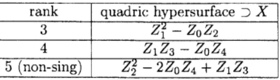
rational quartic curve $X$ in Table 1.

rank quadric hypersurface $\supset X$

3 $\mapsto Z_{1}-Z_{0}\overline{Z_{2}}$

4 $Z_{1}Z_{3}-Z_{0}Z_{4}$ 5(non-sing) $Z_{2}^{2}-$$2\overline{Z_{0}Z_{4}}1$ $Z_{1}Z_{3}$

Table 1: Examples of Quadrics

All the claims except the last one have been already proved in Lemma 3.2. Now we

assume

that there existsashell frame$(E, \sigma)$ of$X$in$W$asinDefinition 2.4. From the homomorphism$\sigma$ : $E^{\vee}arrow$t _{$I_{X/W}\subseteq O_{W}$},

we see that the norrnal bundle$N_{X/W}$ of$X$ in $W$is isomorphic to$E\otimes O_{X}$

.

Putting$U:=Reg(W)$ and the

dualizing line bundle of$W$tobe $K_{W}^{\mathrm{o}}$ (cf. Proposition2.16),

we

have$O(-2)\cong K_{X}\cong K_{U}|_{X}\otimes detN_{X/W}\cong$

($K_{W}^{\mathrm{O}}$ & detE) (&$\mathit{0}\chi$, namely the line bundle $O(-2)$ can be extended to a line bundle_{$L:=K_{W}^{\mathrm{o}}$} (& $detE$

on $W$. By Proposition 2.16 again, we havean isomorphism _$Pic\{W$) $\cong \mathbb{Z}O_{W}(1)$. Then the line bundle $L$

and thereforethe line bundle $O(-2)$ can be extended to amultiple of the tautological line bundle$O_{P}(1)$

of$P$, which contradicts to the fact : _{$O_{X}(1)\cong O(4)$}

.

.

The Case ofcodim(W) $=3$

Next, skipping the most bothersome

case

ofcodim(W) $=2,$

we

proceed to the

case

ofcodirn(W) $=3.$

Then we easily get the following result from Corollary 2.13.

Lemma 3.4 Let$W$ be a pregeometric shell

of

the rationalquartic

curve

$X\subseteq P$ and

of

codimension3 in

P. Then the scheme $W$ coincides with the curve $X$.

.

The Case of codim(W) $=2$

Now we has come to the remaining

case:

codim(W) $=\underline{9}$

.

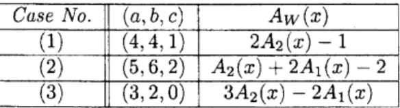
Let us list up all the cases of the triplet $(a, b, c)$ inthe order of handling in the sequel.

Lemma 3.5 Let $W$ be

a

pregeometric shell

of

the rational quartic curve $X\subseteq P$ and

of

codimension2 in P. Then all the

cases

_of

the $Tor$-Betti numbers $(a, b, c)$

of

the minimal graded $S$

-free

resolution$\mathrm{F}_{W}$

,.

and

_of

the Hilbert polynomials are listed in Table 2 below.

Case No. $(a, b, c)$ $A_{W}(x)$

(1) (4, 4,1) $2A_{2}(x)-1$

(2) (5, 6,2)

_A2

$(x)+2A_{1}(x)-$$2$

(3) (3, 2, 0) $3A_{2}(x)-2A_{1}(x)$

Table 2: Betti Numbers and Hilbert Polynomials

Proof. Since the degree of the Hilbert polynomial $A_{W}(x)$ is 2, applying Lemma 3.1, we have the

equa-tions below $((a, b, c)\in\{0,1, \ldots 6\}\cross\{0,1, \ldots 8\}. \cross \{0, 1, \ldots 3\} )$ , whichare easily solved and bring Table

2. $\{$

$1-a+b-c$

$=$ 0 $2a-3b+4c$ $=$ 0 $-a$ $4$ $3b-6c$

7

0 1

Now we will follow the order in Table 2 and handle each case, respectively.

so (1) The Case:(a,$b$,$c$) $=(4,4.1)$

It iseasy to

see

that this

case

never happens.

Since the Hilbert polynomial $Aw(x)$ is A2$(\mathrm{x})-1$, we see that $deg(W)=2.$ On the other hand, we

have $a=4,$ which means thatthere exit four $\mathbb{C}$-linearly independent quadric equations _{$\{G_{1}, G_{2}, G_{3}, G_{4}\}$}

generating the homogeneous ideal$\mathrm{I}_{W}$. Now, using the condition that $W$ is

a

$\mathrm{P}\mathrm{G}$-shell of thecurve $X$, we

recall the proof of Lemma 3.2 andseethat {Gi,$G_{2}$

}

formsa$S$-regular sequence and_{$Y=\{G_{1}=G_{2}=0\}$}

isanarithmetically Cohen-Macaulayclosed subscheme of pure codimensiontwo. Obviously, $X\subset W\subseteq Y,$ $dim(W)=dim(Y)=2,$ and cleg(Yl) $=4.$ Now wetake a primary component $Y_{0}$ of$Y$ containing $X$ and

142

consider $(Y_{0})_{re}d$ after putting the reduced structure on the space $|$}$\mathrm{o}$$|$

.

If de$7((Y\mathrm{o})_{re\mathrm{Z}})$ $\leq 2,$ then after

the process of Lomma 2.15, the one point chordal variety Cd(xo,$(Y_{0})_{r\mathrm{e}d}$) turns out to be alinear variety of dimension 3. Since $X\underline{\subset}(Y_{0})_{red}\subseteq$ Cd(xo,$(Y_{0})_{red}$), we see that the curve $X$ is degenerate, which

is a contradiction. Hence we have $de/$((YQ)$\Gamma ed$) $\geq 3$ and the component $Y_{0}$

can

not contain any main

componentof$W$. Now we have $W\cup$ _(Yo)red $\subseteq Y$ and therefore $deg(Y)\geq 5,$ which is absurd.

..

(2) The Case:(a,$b$,$c$) $=(5,6.2)$

Using a rather delicate argument than the caseabove, we show that thiscase never occurs.

On the Hilbert polynomial, we know that $A_{W}(x)=A_{2}(x)+2A_{1}(x)$-$2=(1/2)x^{2}+(7/2)x+1,$which

implies : $deg(W)=1.$ This shows us that the main component $F$is onlyone and itsstructuresheafas a

primary componentof$W$ is already reduced and isomorphic to the projective plane$\mathrm{P}^{2}(\mathbb{C})$. Since$X\subseteq W$

and $X$ is non-degenerate, we have _$Xl$ $F$ and $Y=X$’ $F\subseteq W,$ where the closed subscheme $Y$ is a scheme theoretic union of the closed subschemes$X$ and $F$. At the generic point $\langle$of the main component

of$W$, $\mathit{0}_{W,\zeta}\cong O_{Y,\zeta}$, which implies that the support of the ideal sheaf_{$I_{Y/W}$} does not contain the generic

point $\zeta$, and therefore $dim(I_{Y/W})\leq 1.$ Then, the Hilbert polynomial of the ideal sheaf

$I_{Y/W}$ is the form

$:\chi(I_{YW}/(x))$ $=px+q$ ($p,$$r\in \mathbb{Z}$and_{$p\geq 0$} ) (cf. [11]). On the otherhand, $XnF$isfinite number of points,

which implies that the Hilbert polynomial is a $\mathrm{c}\mathrm{o}\mathrm{n}\mathrm{s}\mathrm{t}\mathrm{a}\mathrm{n}\mathrm{t}:\chi(\mathrm{O}_{\mathrm{X}\cap \mathrm{F}}\urcorner(x))=k,$ where $k=lengthO_{X\cap F}$. Now

lot usconsider the following two exact sequences:

0 $arrow I_{Y/W}arrow \mathit{0}_{W}arrow \mathit{0}_{Y}arrow 0$

$0arrow O_{Y}arrow O_{X}$ %$O_{F}arrow O_{X\cap F}arrow 0.$ Let us take their Hilbert polynomials, bind them up and get:

$A_{W}(x)$ $=$ $\mathrm{x}\{\mathrm{O}\mathrm{f}\{\mathrm{x}$)) $=\mathrm{x}$

{Of

$\{\mathrm{x}))+\chi(I_{Y/W}(x))$

$=$ $\chi(O_{X}(x))+\chi(O_{F}(x))-\chi(O_{X\ulcorner 1F}(x))+\chi(I_{Y/W}(x))$

$=$ _{$A_{X}(m)+$} $4_{2}(x)-k+px$$+q$

$=$ $4x+1+$(l/2)$(\mathrm{x}+2)(x+1)+px$ $c$ $q-k$

$=$ $(1/2)x^{2}+((11/2)+p)x+(2+q-k)$ .

Comparing the coefficient of the second term in this Hilbert polynomial with that of $Aw(x)$ previously

obtained, we see that (7/2)=((11/2)+p)\geq (ll/7), which is a contradiction.

..

(3) The Case:(a,$b$,$c$) $=(3,2,0)$

Thiscase really occurs and is tllc most interesting fromourview point.

Let us recall: $Ay/(x)=3\mathrm{A}2(\mathrm{x})-2A_{1}(x)$, which implies $deg(W)=3.$ Moreover, the length of the

minimalgraded $S$-free resolution$\mathrm{F}_{W}$

,.

is 2, and therefore arith.$de,pth(W)=$depth(R

$y$) $=5-hds$$(Rw)=$

$5-2=3=dim(R_{W})$ . Thus the homogeneous coordinate ring$R_{W}$ is

an

arithmetically Cohen-Macaulay

ring. Applying Proposition 2.12, we see that the scheme $W$ is a variety of $\triangle$($W$,Aw(x)) $=0$ and of

degree3.

By the structure theoremonthe projective varieties of$\triangle$-genuszero (cf. [6]

or more

classically [12]),

the singular locus Sing(W) of$W$ is alinear space and the variety $W$ is the generalized projectivecone

over a non-singular projective variety $M$ (this can be obtained by a generic linear space section of $W$

which does not meet the linear space Sing(Wl ) of $\triangle$-genus zero withthe vertex at their singular locus.

Since $dim(W)=2,$ we haveonlytwocases : (3-1) $dim(Sing(W))=-1$ (namely $W$ is non-singular) and

the non-singular variety $M$ is $W$ itself; or (3-2) $dim(Sing(W))$ $=0$ (namely Sing(W) $=\{p_{0}\}$) and the non-singular variety$M$ is a rational normal cubiccurve.

Moreover,the structure theorem says that in thecaseof(3-1) above, the polarizedvariety $(W, O_{W}(1))$

is

a

rational scroll $(\mathrm{P}(E), O_{\mathrm{P}(E)}(1))$, where the vector bundle$E$istheone overarationalcurve$B=\mathrm{P}^{1}(\mathbb{C})$

and of the form: $E\cong O_{\mathrm{P}^{1}(\mathrm{C})}(2)\oplus O_{\mathrm{P}^{1}(\mathbb{C})}(1)$, the ample line bundle $o_{\mathrm{P}(E)}(1)$ is the relative tautological

line bundle of the projective bundle$\mathrm{P}(E)arrow B$ determined from the ample vector bundle $E$. In te rns of rational ruled surfaces, this variety $W$is isomorphic to $\Sigma_{1}$, arational ruled surface of degree 1 and is

embedded by a linearsystem 2$f+C_{1}|$

.

Ontheother hand, in thecaseof(3-2), the blow-up$q$ : $\overline{W}arrow W\subseteq P$of the variety$W$ atthevertex$p_{0}$ is obtained by$\overline{W}\cong \mathrm{P}(O_{1\mathrm{I}^{\nu 1}(\mathbb{C})}(3)\oplus O_{\mathrm{P}^{1}(\mathrm{C})})$ and byanatural homomorphism$\oplus^{5}\mathit{0}_{\mathrm{P}^{1}(\mathbb{C})}arrow O_{1\mathrm{P}^{1}(\mathrm{C})}(3)\oplus O_{1\mathrm{P}^{1}(\mathrm{C})}$

on a rational curve $B=\mathrm{P}^{1}(\mathbb{C})$. This variety $W$ is isomorphicto $\Sigma_{3}$, a rational ruled surface of degree 3

and the morphism $q$ : $\overline{W}arrow W\subseteq P$is given by

a

linear system $3f+C_{3}|$.

Let us summarize these two

cases

in the following Table 3 and proceed to study how the curve $X$ is

embedded in $W$ in each

case.

Case No. $dim(S^{\cdot}g(W))$ $\overline{W}$

or $\mathrm{Y}$

$1\mathrm{i}1$ear system (morph.)

(3-1) -1 (on-sing) $W\cong$$\Sigma_{1}$ $|2f+C_{1}|$ (embedding)

(3-2) 0 $\overline{W}\cong$

$\mathrm{g}_{3}$ $|3f+C_{3}|$

Table 3: Cases of $(W, O_{W(}’1))$

\ldots The Case (3-1)

Nowwe

assume

thatthe variety $W$ is isomorphic to the ruledsurface $\Sigma_{1}$ and embedded into$P$ by the

linear system $|2f+C_{1}|$. Since$X\in|uf+vC_{1}|$ for

some

integer$u$$\mathrm{t}^{\mathrm{t}}$ the fact: $deg(X)=4$and theLemma

2.2 (2.2.3),

we

have : $(u, v)=(3,1)$ or $(2, 2)$_. Let us take

a

blow-down morphism $b$:II $arrow \mathrm{P}^{2}(\mathbb{C})=Y$ of

contracting the exceptionalcurve$C_{1}$toapoint$p\in Y.$ Then the pull-back : $b^{*}O_{\mathrm{P}^{\underline{\circ}}(\mathbb{C})}(1)$ of the tautological

ample line bundle ofthe projective plane $Y$corresponds to the linear system $|f+C_{1}$$|$. Thus, if the curve

$X\in|3f+C_{1}|$, applying the projection formula tothe curve $X$ with respect to the morphism $b$, and the computation : $X.(f+C_{1})=3$, $X.C_{1}=2$ show that the the curve $X$ comes from a singular irreducible

and reduced cubic plane curve passing through the point $p$. Consideringthat 3$f+C_{1}=(2f+C_{1})+f,$

namely

a sum

of the ample divisor 2$f+C_{1}$ and

an

(effective) nefdivisor $f$, we see that the

curve

$X$ is a nef divisor (an ample divisor).

By the similar argument, if the

curve

$X\in|2f+2C_{1}|$, we

see

that the curve $X$ comes from a

non-singular conic which does not pass through the point $p$

.

To see the curve $X$ is

a

nef divisor (N.B. not

ample e.g. $X.C_{1}=0$), we have onlyto apply the projection formula to atest curvewith respect to the

morphism $b$since

$X\in|/\mathrm{t}’ O_{\mathrm{P}}\circ\sim(\mathbb{C})(2)|$.

\ldots The Case (3-2)

Next we consider the

case

:the $\mathrm{b}\mathrm{l}\mathrm{o}\mathrm{w}\underline{- \mathrm{u}}\mathrm{p}\overline{W}$of the variety _$W$ at the vertex

$p_{0}$ is isomorphic to the ruled surface $\Sigma_{3}$ and the morphism

$q$ : $Warrow W\subset P$ is given by the linear system $|3f+C_{3}|$. Now,

taking the strict transform$q^{-1}(X)$ of thecurve$X$ via the morphism$q$, weseek the integers $u$and $v$such

that $q^{-1}(X)\in|uf+vC_{3}|$. _{Then the condition $deg(X)=4$} means $q^{-1}(X).(3f+C_{3})=4.$ Since the

curve

$q^{-1}(X)$ is irreducible, we can apply Lemma 2.2 (2.2.3) to this case and get $(\iota x, \tau))=(4,1)$. Then

X.C3 $=(4f+C_{3}).C_{3}=4-$$3$ _$=1,$ whichshows the curve$X$ passes simply through the vertex$p_{0}$.

4

Existence

Now let

us

show the existence of the three

cases

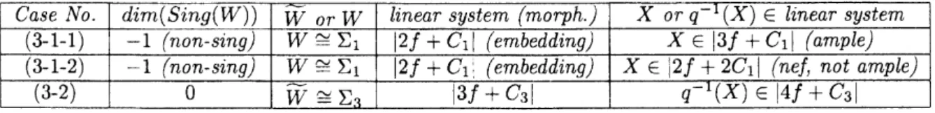
above and summarize the classification ofthe case

144

Proposition 3.6 Let $X$ be a non-degenerate quartic

nor

rmal

curve

in $P=\mathrm{P}^{4}(\mathbb{C})=$ Proj(S) and $Wa$

pregeometric shell

_of

$X$ with codim(W) $=2.$ Then $W$ isreduced and irreducible and a variety

of

A-genus

zero. The homogeneous coordinate ring$R_{W}$

of

$W$ has a minimal graded$S$

-free

resolution$\mathrm{F}_{W}$

,.

with the

$Tor$-Betti numbers $(3, 2_{\backslash }0)$

.

There are three possible cases satisfying these properties as in Table

4.

Case No. $d.m(S^{\cdot}/(W))$ $W$ or$W$ $l$. ear $sytem(mo h.)$ $X$ or$q^{-\mathrm{I}}(X)\in-$llnear system

(3-1-1) -1 (on-s. $g$) $\cong\Sigma_{1}$ $|\mathit{2}f+C\mathrm{l}$$|$ (embeddi $g$) $X\in|37$ $+C_{1}|$ (ample)

(3-1-2) -1 $(0-\cdot. g)$ $W\cong\Sigma_{1}$ $|2f+C\mathrm{l}$$|(emb\overline{edd}. g)$ _{$X\in|2f+2C_{1}|$} ($nef$, not ample)

(3-2)

–0

$–\cong\Sigma$ $|3f+C_{3}|$ $q^{\overline{-1}}(X)\in|4f+C_{3}|$ Table

_4:

Cases

_of

a

_surface

W and a curve$X$

Conversely, there exista non-singularprojective

_surface

$W$ and a non-singularprojective curve$X$ on$W$

which satisfy the conditions in Table

₄

above. Moreover, once

_if

the

_surface

$W$ and the curve $X$ on $W$

are given asin Table

₄

above, then the

_surface

$W$ is always apregeometric shell

of

the curve $X$ (cf. also

\S 4

$\cdot$).

Proof. It is enough to show the existence part of the claim above. If

we

do not

assume

the condition of “pregeometricshells”,, Lemma 2.2 (2.2.3) shows theexistences of pairs ofanon-singular projective curve

anda non-singularprojectivesurface: $X\subset W$in $P=\mathrm{P}^{4}(\mathbb{C})$ asin Table 4. Then, the curve $X$ is a curve

ofdegree 4 and thesurface $W$ isofdegree 3. Bythis construction, thesurface $W$is alinearlynormal, i.e.

a natural map $H^{0}(P, O_{\mathrm{P}}(1))arrow H^{0}(W, O_{W}(1))$ is surjective. On the non-degeneracy of $X$, using Table

4, we can check it easily by computing $H^{0}(W, I_{X/W}(H))\cong H^{0}(W, O_{W}(-X+H))$ $=0$ (if $W\cong\Sigma_{1}$) or

$H^{0}(\overline{7\overline{V}}, I_{q}1(X)/\tilde{W}(q^{*}H))\cong H^{0}(\overline{W}, O_{\overline{W}}(-q^{-1}(X)+q^{*}H))=0$ (if $\overline{W}\cong$

E3). This also shows the linear normalityof the rational curve $X$ (adjunctionformula and Lemma 2.2 (2.2.4)).

Let us show that the surface $W$ is apregeometric shell of$X$ in these three cases. In every case, both

the surface $W$ and the curve $X$ are varieties of$\triangle$-genera zero. Now we refer to the book [6] and apply

its results: (4.12) Corollary and the argument of (5.1), which imply that both varieties $X$ and $W$ are

with metically Cohen-Macaulay. Then the result of [5] showsthat the homogeneous coordinate rings $R_{W}$

has 2-lincar minimal graded $S$-free resolution. Applying Proposition 2.5 (2.5.8), we seethat the surface

It is a pregeometric shell of$X$. $\mathrm{I}$

The argunent in the proofof Proposition 3.6 brings also the following useful result.

Corollary 3.7 Let $V\subset W$ be closed subschemes

of

$P=\mathrm{P}^{N}(\mathbb{C})$. Assume that the scheme $V$ is

non-deqcneratc and the scherne $W$ is linearly normal and

of

a variety

of

$\triangle$-genus zero. Then the variety $W$

is a pregeometric shell

_of

$V$.

Corollary 3.8 Let $V\subset P=\mathrm{P}^{N}(\mathbb{C})$ be a non-degenerate, linearly no rmal closed subvariety

of

codimen-sion$r$ and

of

$\triangle$-genus zero. Then, there is

a

chain

of

varieties:

$V=W_{0}\subset W_{1}\subset W_{2}\subset\cdots\subset W_{k}\subset\cdots\subset W_{r}=P,$

where the variety $W_{k}$ $(k=0,1, \cdots, r)$ is apregeometric shell

of

$V$ with $cod_{i}m(W_{k}, P)$ $=r-k.$

Proof. Starting from the variety $V$, we first construct inductively a chain of varieties $\{W_{k}\}_{k=0}^{r}$ with

$\triangle$-genus zero. Asan induction hypothesis, we assume