Local and global well-posedness for the KdV equation at the critical regularity (Nonlinear evolution equations and mathematical modeling)

Local and

global well-posedness for the KdV equation

at the

critical

regularity

京都大学大学院理学研究科 岸本展 (Nobu Kishimoto)

Department of Mathematics, Kyoto University

1. Introduction

In this note,

we

study the Cauchy problem of the $KdV$ equation:

$\{\begin{array}{ll}\partial_{t}u+\partial_{x}^{3}u=\partial_{x}(u^{2}), u:[-T,T]\cross \mathbb{R}arrow \mathbb{R} or \mathbb{C},u(0, x)=u_{0}(x). \end{array}$ (1)

This is a survey of the author’s papers [13, 14], and we refer to them for detailed

discussion.

The

$KdV$ equation

was

originally derived by Korteweg and de Vries [15]

as

a model

for the propagation ofshallow waterwaves along a canal. It appears in various phases

of mathematical physics;

see

[7] for

a

number of applications. It is also well-known

as one

of the simplest PDEs that have complete integrability.

We shall consider local and global well-posedness of (1) with initial data given in

Sobolev spaces $H^{s}(\mathbb{R})$ defined via the

norm

$\Vert\phi\Vert_{H}$

。

$(R)^{;=}\Vert\langle\cdot\}^{s}\hat{\phi}\Vert_{L^{2}(R)}$,

where $\wedge$

denotes the Fourier transform and $\langle\cdot)$ $:=(1+|\cdot|^{2})^{1\prime 2}$

.

We say the Cauchy

problem is locally well-posed in $H^{s}$ if for any initial datum $u_{0}\in H^{s}$, there exists a

time of local existence $T=T(\Vert u_{0}\Vert_{H^{t}})>0$ and the solution in $C([-T, T];H^{s})$ which

is unique in

some

sense

and depends continuously on the datum. If the above $T$

can

be chosen arbitrarily large, we say the Cauchy problem is globally well-posed in $H^{s}$

.

Note that it does not make any differences whether we take $[-T,T]$

or

$[0, T]$

as

the

interval of local existence, because the $KdV$ equation has time reversal symmetry.

Our main results

are

the local well-posedness of (1) and the global well-posedness

of real-valued (1) in $H^{-3\prime 4}(\mathbb{R})$

.

We

now

review the iteration method for proving the local well-posedness and clarify

the meaning of a ‘solution’ to the Cauchy problem.

First,

we

replace the Cauchy problem with the corresponding integral equation via

the Duhamel formula,

$u(t)=e^{-t\partial_{x}^{3}}u_{0}+ \int_{0}^{t}e^{-(t-t’)\partial_{x}^{3}}\partial_{x}(u(t’)^{2})dt’$, $t\in[-T,T]$, (2)

We then put the right hand side of (2) $\Phi_{u_{0}}(u)(t)$ and try to show that $\Phi_{u_{0}}$ is a

contraction map on a certain Banach space $S_{T}^{s}$ embedded in $C([-T, T];H^{s})$

.

Note

that the operator $\Phi_{u_{0}}$ is for now defined only

on

smooth functions (with enough

decay at spatial infinity). For instance, ifwe consider negative regularities $s<0$, we

will fail to define the quadratic nonlinear term for all $u\in C([-T, T];H^{s})$

.

Thus, it

is important to find a function space $S_{T}^{s}$ so that the domain of $\Phi_{u_{0}}$ can be extended

appropriately to all functions in this space.

For the contractiveness of the operator $\Phi_{u_{0}}$, the following linear and bilinear

esti-mates

are

basically needed:

$\Vert e^{-t\partial_{x}^{3}}u_{0}\Vert_{S_{T}^{\epsilon}}\leq C\Vert u_{0}\Vert_{H^{S}}$

,

$\Vert\int_{0}^{t}e^{-(t-t’)\partial_{x}^{3}}\partial_{x}(u(t’)v(t’))dt’\Vert_{S_{T}^{s}}\leq C\Vert u\Vert_{S_{T}^{s}}\Vert v\Vert_{S_{T}^{\epsilon}}$

.

Once these estimates

are

established with a Banach space $S_{T}^{s}$ in which smooth

func-tions are dense, definition ofthe Duhamel term in $\Phi_{u_{0}}$ will be extended to the whole

$S_{T}^{s}\cross S_{T}^{s}$ in the unique continuous sense. Then, we consider a function $u$ as asolution

to the Cauchy problem if $u$ satisfies the equation $u=\Phi_{u_{O}}(u)$ in $S_{T}^{s}$

.

It is easy to

verify that such a solution is the unique limit in $S_{T}^{s}$ of smooth solutions starting from

initial data smoothly approximating the original datum $u_{0}$ in $H^{s}$

.

The above two estimates are actually enough to show that $\Phi_{u0}$ is contractive on

$\{u\in S_{T}^{s}|\Vert u\Vert_{S_{T}^{\epsilon}}\leq 2C\Vert u_{0}\Vert_{H^{\epsilon}}\}$ if$u_{0}$ is sufficiently small. We thus obtain a solution

as the uniquefixed pointof$\Phi_{u_{0}}$, and the Lipschitz continuous dependence of solutions

on

data also follows naturally. Note that the$KdV$ equation has thescaling invariance,

that is, the scaling transform

$u(t, x)$ $\mapsto$ $u^{\lambda}(t, x)$ $:=\lambda^{-2}u(\lambda^{-3}t, \lambda^{-1}x)$, $\lambda>0$

maps a solution of (1) to the solution with initial datum $u_{0}^{\lambda}(x):=\lambda^{-2}u_{0}(\lambda^{-1}x)$

.

Since we have

$\Vert u_{0}^{\lambda}\Vert_{H^{s}(\mathbb{R})}=O(\lambda^{-3’ 2-\min\{0,s\}})$

as $\lambdaarrow\infty$, the problem for general initial data is reduced to solving the equation

on

the time interval [-1, 1] for any sufficiently small data as long as we treat $s>-3/2$

.

From

now

on,

we

consider the

case

$T=1$

.

We have

seen

that the linear solution $e^{-t\partial_{\alpha}^{3}}u_{0}$ is defined clearly through the spatial

Fourier transform; however, it is instructive to compute the space-time Fourier

trans-form of the linear solution. The result for a smooth $u_{0}$ is $c\delta(\tau-\xi^{3})\hat{u_{0}}(\xi)$, where $\delta$

denotes the Dirac delta function. We find a remarkable property of the linear solution

that it is supported in the space-time frequency space

on

the cubic

curve

$\{\tau=\xi^{3}\}$

.

In order to take advantage of the space-time Fourier transform in the context of

nonlinear equations, we need to deal with a solution

as

a function

on

the entire space

$\mathbb{R}^{2}$ rather than on

bump function $\psi$ on $\mathbb{R}$ satisfying _{$\psi\equiv 1$} on [-1, 1] and $supp\psi\subset[-2,2]$, and then

seek a solution to the global-in-time integral equation

$u(t)= \psi(t)e^{-t\partial_{x}^{3}}u_{0}+\psi(t)\int_{0}^{t}e^{-(t-t’)\partial_{x}^{3}}\partial_{x}(u(t’)^{2})dt’$ , $t\in \mathbb{R}$,

instead of the previous local-in-time equation. A. simple computation implies that

the space-time Fourier transform of the truncated linear solution $\psi(t)e^{-t\partial_{x}^{3}}u_{0}$ with

a smooth $u_{0}$ is equal to $\hat{\psi}(\tau-\xi^{3})\hat{u_{0}}(\xi)$, which is now a smooth function mainly

supported

near

the cubic

curve

(in fact it is rapidly decreasing in the variable $\tau-$

$\xi^{3})$

.

As long

as

the nonlinear equation

can

be thought of

as a

perturbation of the

linear equation, it is expected that the nonlinear solution also concentrates near the

characteristic hypersurface.

From this point ofview, it is quite natural to introduce the Bourgain spaces $X^{s,b}$,

or the Fourier restriction spaces, defined as the completion of space-time Schwartz

functions with respect to the

norm

$\Vert u\Vert_{X^{s,b}}:=\Vert\langle\xi\rangle^{s}\langle\tau-\xi^{3}\rangle^{b}\tilde{u}(\tau, \xi)\Vert_{L_{\tau,\zeta}^{2}}$,

where $\tilde{u}$ denotes the space-time Fourier transform of

$u$

.

If the real parameter $b$ is

greater than 1/2, then the continuous embedding $X^{s,b}arrow C(\mathbb{R};H^{s})$ holds. In this

case, $X^{s,b}$ effectively captures functions supported in frequency

near

the cubic

curve

from the space $C(\mathbb{R};H^{s})$

.

Note also that $X^{s,b}$

can

be regarded

as

theproduct Sobolev

spaces twisted by the linear evolution; in fact, we have

$\Vert u\Vert_{X^{\iota,b}}=\Vert e^{t\partial_{x}^{3}}u(t)\Vert_{H_{t}^{b}(H_{x}^{*})}$

.

The Bourgain spaces $X^{s,b}$, named after J. Bourgain who introduced it to study the

nonlinear Schr\"odinger and $KdV$ equations [2, 3], provided substantial progress in the

well-posedness theory for a wide variety of nonlinear dispersive equations. Especially,

it is a quite powerful tool to establish the local well-posedness in Sobolev spaces with

very low (perhaps negative) regularities.

If the space $X^{s,b}$ is used for the resolution space $S^{s}$, the estimates required to make

$\Phi_{u_{O}}$ contractive will be described

as

$\Vert\psi(t)e^{- t\partial_{x}^{3}}u_{0}\Vert_{X^{s,b}}\leq C$

II

$u_{0}11_{H^{s}}$, (3) $\Vert\psi(t)\int_{0}^{t}e^{-(t- t’)\partial_{x}^{3}}\partial_{x}(u(t’)v(t’))dt’\Vert_{X^{\epsilon,b}}\leq c\Vert u\Vert_{X^{\text{。},b}}\Vert v\Vert_{X^{\text{。},b}}$

.

(4)

We usually divide the second estimate (4) into the linear Duhamel estimate

and the bilinear estimate

$\Vert\partial_{x}(uv)\Vert_{X^{s,b-1}}\leq C\Vert u\Vert_{X^{s,b}}\Vert v\Vert_{X^{\epsilon,b}}$

.

(6)

The choice of auxiliary space $X^{s_{2}b-1}$ for nonlinearity

seems

natural if

we

recall that

theparameter $b$denotesthe regularity with respect to thedifferential operator $\partial_{t}+\partial_{x}^{3}$,

and that the solutions $u=(\partial_{t}+\partial_{x}^{3})^{-1}\partial_{x}(u^{2})$ should be in $X^{s,b}$

.

Then, it is enough for the local well-posedness in $H^{s}$ to establish the estimates (3),

(5), and (6). It turns out that two linear estimates (3) and (5) hold for any $s\in \mathbb{R}$

with appropriate values of$b$;

see

[8] for instance. Incontrast, the bilinear estimate (6)

is known to fail for any $b$ if we consider regularities below

a

certain threshold. This

fact suggests that if the data become rougher, the nonlinear effect will get stronger

and the nonlinear equation will behave less as a perturbation of the linear equation.

Therefore, the bilinear estimate (6) controlling nonlinearity is directly connected to

the well-posedness and plays a crucial role in the iteration argument.

2.

Previous

results

and the

main

theorem

The Cauchy problem (1) has been extensively studied. We first recall that Kenig,

Ponce, and Vega [11] established the bilinear estimate (6) for $s>-3/4$ with some

$b>1/2$, which implies the local well-posedness of (1) in the corresponding regularity.

Their local result was improved to the global well-posedness in $H^{s}(\mathbb{R})$ with $s>-3/4$

in the real-valued case by Colliander, Keel, Staffilani, Takaoka, and Tao [6]. The

proof was based on the I-method, which we shall review in Section 5.

It is natural to try to verify the bilinear estimate for $s\leq-3/4$ if one wishes to

obtain the well-posedness for that regularity. However, it is known that (6) fails for

any $b\in \mathbb{R}$ if$s\leq-3/4$ ([11, 17]). Moreover, when $s<-3/4$ the data-to-solution map

for (1) fails to be uniformly continuous as a map from $H^{s}$ to $C_{t}(H_{x}^{s})$ ([12, 4]). This

result does not necessarily imply the ill-posedness of the Cauchy problem, but the

iteration method would naturally provide the Lipschitz continuity, so it will not work

for regularities $s<-3/4$ . It is an important open problem whether the local

well-posedness with a merely continuous data-to-solution map holds in these regularities.

We

now

focus on the

case

$s=-3/4$

.

As

seen

above, this is the critical regularity for

the iteration method (but far above the scaling critical regularity $s=-3/2$). Since

we do not have the bilinear estimate in $X^{-3’ 4,b}$, we have to iterate in a different

space,

or

abandon the direct iteration method, to obtain well-posedness in $H^{-3\prime 4}$

.

The latter approach

was

taken in [4]. They obtained the local-in-time result for (1)

in $H^{-3’ 4}(\mathbb{R})$ by combining (slightly modified) Miura transform with the

correspond-ing local well-posedness for the modified $KdV$ equation in $H^{1’ 4}(\mathbb{R})$ obtained in [10].

The Cauchy problem of the

_modified

$KdV$ equation,

is also well-studied and linked with the $KdV$ equation through the Miura transform;

if$v$ is a smooth solution to (7), then $u$ $:=c_{1}\partial_{x}v+c_{2}v^{2}$ with suitable constants $c_{1},$$c_{2}$

solves the $KdV$ equation. Since the Miura transform acts roughly

as

a derivative,

many results for $KdV$ have counterparts for modified $KdV$ at

one

higher regularity;

for instance, the regularity threshold for validity of the iteration method is $s=1/4$

,

exactly

one

higher than $s=-3/4$ for $KdV$

.

We point out that the above result for $KdV$ in $H^{-3’ 4}$ is relatively weak, compared

with that for $s>-3/4$

.

Firstly, the uniqueness of solutions

was

obtained only in

the image of the Miura transform. In fact, for the

case.

$s>-3/4$ it

was

shown that

solutions

are

unique in $X^{s,b}$

.

Since the Miura transform is

a

nonlinear mapping,

we

find it not

so

easy to analyze the structure of its image,

or

verify whether

a

given

function is in its image or not. Secondly, we do not have the control of their local

solutions in a function space well adapted to the I-method, such

as

$X^{s,b}$

.

This is why

the global well-posedness for real-valued (1) in $H^{-3\prime 4}(\mathbb{R})$

was

left open.

Iilrom this point ofview, it is quite interesting to investigate the strong local

well-posedness for (1) in $H^{-3\prime 4}(\mathbb{R})$ by the iteration method. Our main result precisely

deals with this issue. Of course, we have to change the working space from $X^{-3\prime 4,b}$

.

We shall constmct a Banach space $X$ as the working space $S^{-3’ 4}$, which is

some

Besov-like generalization of the Bourgain space $X^{-3\prime 4,1\prime 2}$ with slight modification

in low frequency. See the definition in the next section. The space $X$ possesses the

bilinear estimate similar to (6), but fails to be embedded into $C(\mathbb{R};H^{-3\prime 4})$, which

forces us to introduce

an

auxiliary space $Y$ defined by the

norm

$\Vert u\Vert_{Y}:=\Vert\langle\xi\}^{-3’ 4}\tilde{u}\Vert_{L_{\zeta}^{2}(L_{\tau}^{1})}$

.

This space $Y$ has also appeared in

a

number of previous works (originally in [8]). For

these spaces we have the following bilinear estimate:

Proposition 1. We have

$\Vert\langle\partial_{t}+\partial_{x}^{3}\rangle^{-1}\partial_{x}(uv)\Vert_{X}+\Vert\langle\partial_{t}+\partial_{x}^{3}\rangle^{-1}\partial_{x}(uv)\Vert_{Y}\leq C\Vert u\Vert_{X}\Vert v\Vert_{X}$,

where $\langle\partial_{t}+\partial_{x}^{3}\rangle^{-1}$ is the space-time Fourier multiplier corresponding to $\langle\tau-\xi^{3})^{-1}$

A standard iteration argument then implies

our

main theorem.

Theorem 1. The Cauchy problem (1) (real-valued orcomplex-valued) is locally

well-posed in$H^{-3’ 4}(\mathbb{R})$

.

In particular, solutions

are

unique in $X$ to be

defined

in Section 3.

We remark that the uniqueness in the above theorem is precisely as follows: the

solutions of (1) on the time interval $[-T,T]$ are unique in the class $X_{1-T,T]}$, where

functions in $X$, which is equipped with the restricted norm

$\Vert u\Vert_{X_{I}}$ $:= \inf\{\Vert U\Vert_{X}|U\in X,$ $U(t)=u(t)$ for $t\in I\}$

.

We also

use

this restricted

norm

for a global-in-time function $u$ under the convention

of $\Vert u\Vert_{X_{I}}:=\Vert u|_{t\in I}\Vert_{X_{I}}$

.

This theorem combined with the I-method yields the global results. Since

our

function space $X$ is very close to the usual Bourgain space $X^{s,b}$ (in fact satisfies the

embedding $X^{-3\prime 4,b}arrow Xarrow X^{-3’ 4,1’ 2}$ _{for any $b>1/2$), proof is almost identical}

with the

case

of $X^{s,b}$ for $s>-3/4$

.

Theorem 2. The real-valued Cauchyproblem (1) is globally well-posed in $H^{\sim 3\prime 4}(\mathbb{R})$

.

Note that these global results do not hold for the complex-valued

case.

In fact,

several finite-time blow-up solutions have been discovered. For instance, see [1] and

references therein.

In the next section,

we

will discuss how to construct the space $X$ which yields

the crucial bilinear estimate. The proof of Proposition 1 is quite complicated,

so we

refer to [13] for it. In Section 4, we will show outline of the proof for Theorem 1,

especially for the uniqueness of solutions. Section 5 will be devoted to a review of

the I-method. We will omit the details for the proof of Theorem 2 and refer to [6].

In the last section, we will recall a recent result by Guo [9] and compare it with

ours.

3.

Construction

of the working

space

Let

us

recall some counterexamples to the bilinear estimate in $X^{-3\prime 4,b}$,

$\Vert\partial_{x}(uv)\Vert_{x-3/4,b-1}\leq C\Vert u\Vert_{x-3/4,b}\Vert v\Vert_{x-3\prime 4,b}$ , (8)

and then

see

how to modify the Bourgain spaces so that these examples may be

suitably controlled.

We first prepare

some

notations for convenience. Let us fix a smooth function

$q_{0}:\mathbb{R}arrow[0,1]$ which is equal to 1 on $[-5/4,5/4]$ and supported in

$[-85,85]$

.

For

$N>0$ and $j=1,2,$ $\ldots$, define

$q_{N}(\xi):=q_{0}(\dot{N})-q_{0}(N)$, $p_{0}:=q_{0}$, $p_{j}:=q_{2^{j}}$,

and then denote the Fourier multipliers with respect to $x$ corresponding to $q_{0},$ $q_{N},$ $p_{0}$,

and $p_{j}$ by $Q_{0},$ $Q_{N},$ $P_{0}$, and $P_{j}$, respectively. Note that $\{P_{j}\}_{j=0}^{\infty}$ is

an

inhomogeneous

Littlewood-Paley decomposition, and that QN with $N>0$ is thefrequency-localizing

operator satisfying $suppq_{N}\subset\{\frac{5N}{8}\leq|\xi|\leq\frac{8N}{5}\},$ $q_{N}\equiv 1$ on $\{\frac{4N}{5}\leq|\xi|\leq\frac{5N}{4}\}$

.

Proposition 2 ([11]). Let $b\in \mathbb{R}$, then there exists $c>0$ such that the following holds.

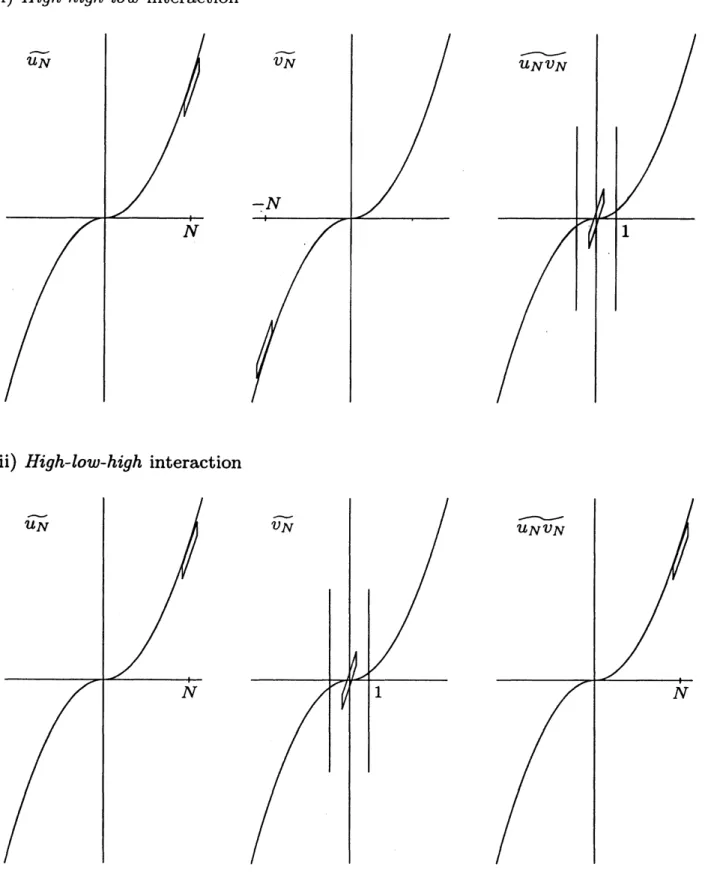
(i) For any $N\gg 1$, there exist $u_{N},$$v_{N}$ satisfying $Q_{N}u_{N}=U_{N}$, $QNVN=v_{N}$, and

$\Vert Q_{0}\partial_{x}(u_{N}v_{N})\Vert_{X^{-3\prime 4,b-1}}\geq cN^{\S b-\S}\Vert u_{N}\Vert_{x-3/4,b}\Vert v_{N}\Vert_{X^{-3/4,b}}$

.

(ii) For any $N\gg 1$, there exist $u_{N},v_{N}$ satisfying $Q_{N^{U}N}=U_{N},$ $Q_{0}v_{N}=v_{N}$, and

$|1\partial_{x}(u_{N}v_{N})\Vert_{x- 3’ 4,b- 1}\geq cN^{\S\# b}\langle N\}^{-}$ ’

11

$u_{N}\Vert_{X-3\prime 4,b}$

II

$v_{N}$

I

$x- 3\prime 4,b$

.

This proposition says that (8) fails to hold for $b>1’ 2$ (from $(i)$), and for $b<1/2$

(from (ii)). These examples

are

sketched in Figure 1. We observe that the example

in (i) consists ofhigh-frequency functions supported in the frequency space along the

curve $\tau=\xi^{3}$, and their product (or, in frequency, their convolution) is concentrated

near

the frequency origin (thus in the low-frequency region). We call such

interac-tions high-high-low. On the other hand, the example in (ii) is the interaction between

functions of high frequency and low frequency, which produces a high-frequency

com-ponent near the curve, so we call it high-low-high interaction.

The bilinear estimate (8) also fails in the

case

$b=1/2$, but the divergence order is

logarithmic in $N$ rather than power in $N$

as

Proposition 2.

Proposition 3 ([17]). Let $0<\alpha<1/2$, then there exists $c>0$ such that the following

holds: For any $N\gg 1$, there exist $u_{N},$$v_{N}$ satisfying $QNUN=u_{N},$ $Q_{N}v_{N}=v_{N}$, and

$\Vert Q_{0}\partial_{x}(u_{N}v_{N})\Vert_{X^{-3/4,-1\prime 2}}\geq c(\log N)^{\alpha}\Vert u_{N}\Vert_{x-3/4,1/2}\Vert v_{N}\Vert_{x-3\prime 4,1/2}$

.

As sketched in Figure 2, this example of high-high-low type is much

more

com-plicated than the previous

one.

We point out that the high-frequency function is

supported also in the region distant from the

curve

$\tau=\xi^{3}$ in contrast to the

coun-terexamples in Proposition 2. In fact, $u_{N}$ consists of $\epsilon\log N$ components

dyadi-cally supported away from the

curve

$(0<\epsilon\ll 1)$. Each of these components $u_{N_{2}j}$

$(1\leq j\leq\epsilon\log N)$, which has

some

positive $X^{-3\prime 4,1\prime 2}$

norm

$a_{j}$, interacts with $v_{N}$ and

outputs the component, whose norm is

Il

$\partial_{x}(u_{N_{2}j}v_{N})||_{x-3/4,-1/2}>a_{j}\sim\Vert V_{N}||_{X^{-3/4,1/2}}$, at

almost the

same

part of the low-frequency region $\{|\xi|\leq 1\}$

.

The

norm

of the total

output is then at least

11

$v_{N} \Vert_{x-3’ 4,1/2}\sum a_{j}$, while the norm of $u_{N}$ is equal to the $\ell^{2}$

sum

of those of$u_{N,j}’ s;\Vert u_{N}\Vert_{X^{-3’ 4,1/2}}\sim(\sum a_{j}^{2})^{1\prime 2}$

.

Putting $a_{j}=j^{\alpha-1}(0<\alpha<1’ 2)$

for instance, we have the divergence of $O((\log N)^{\alpha})$

.

We have seen that the bilinear estimate in $X^{-3’ 4,b},$ (8), failsforany $b\in \mathbb{R}$, and that

the divergence in the case $b=1/2$ is logarithmic, better than the other

cases.

There-fore, we shall start from $X^{-3\prime 4,1\prime 2}$ and modify it to endure the nonlinear interaction

described in Proposition 3.

In the analysis with the Bourgain spaces, in fact, logarithmic divergences of

non-linear estimates often occur in such a limiting regularity. One standard way to avoid

(i) High-high-low interaction

(ii) High-low-high interaction

Figure 1. Two typical nonlinear interactions described in Proposition 2. In the context of the bilinear estimate (8) for $b\neq 1/2$, they produce some power

Figure 2. The example of high-high-low interaction described in Proposition 3, which breaks the bilinear estimate in $X^{-3\prime 4,1\prime 2}$ with logarithmic divergence.

This is similar to the space $B_{2,1}^{1/2}(\mathbb{R})$

as

a modification of $H^{1\prime 2}(\mathbb{R})$, which has many

good properties such

as

the embedding into the space of bounded continuous

func-tions. $\ell^{1}$-Besov structure is also convenient for the summation of dyadic frequency

pieces: For example, if

we

have a frequency-localized bilinear estimate

$\Vert B(P_{j}u, P_{k}v)\Vert\leq C\Vert P_{j}u\Vert\Vert P_{k}v\Vert$

for

some

bilinear operator $B$, then the bilinear estimate

11

$B(u,v)$

Il

$\leq C\Vert u\Vert\Vert v\Vert$

immediately follows from the triangle inequality and the $\ell^{1}$ nature of the norm.

Such Besov-type Bourgain spaces were used first in the context of the

wave

map

equations ([18]), and have appeared in a number of literature.

In our context, the $\ell^{1}$-Besov Bourgain spaces $X^{s,b,1}$ is defined by the norm

$\Vert u\Vert_{X^{\epsilon,b,1}}:=(\sum_{j=0}^{\infty}2^{2sj}(\sum_{k=0}^{\infty}2^{bk}\Vert p_{j}(\xi)p_{k}(\tau-\xi^{3})\hat{u}\Vert_{L_{\tau,\zeta}^{2}})^{2})^{1\prime 2}$

The usual $X^{s,b}$ norm is equivalent to the above norm with the $\ell_{k}^{1}$

sum

replaced by

$\ell_{k}^{2}$

.

We see that $X^{s,b,1}$ is slightly stronger than $X^{s,b}$

.

Note that the counterexample in Proposition 3 can be well controlled ifwe

measure

$\overline{X^{-3\prime 4,1’ 2+\epsilon}X^{-3\prime 4,1\prime 2-\epsilon}X^{-3\prime 4,1’ 2}X^{-3\prime 4,1’ 2,1}X_{*}}$

high-high-low $Prop2(i)N^{\alpha}$ $(\log NProp3^{\alpha}$ $f_{rop4(i)}^{\log N)^{\alpha}}$

Prop 2 (ii)

high-low-high $N^{\alpha}$

$i_{r\circ p4}^{\log N}/ii$

)

$\alpha$

$f_{rop4}^{1oN}l_{ii)}^{\alpha}$

Table 1. Various divergences in the bilinear estimates for $s=-3/4$

.

the bottom regularity, similar issues may arise, and the space $X^{s,1\prime 2,1}$ is considered

generally

as a

good substitute for $X^{s,1’ 2}$

.

However,$\cdot$

for the $KdV$ _case,

_{we can}

_not

restore the bilinear estimate in $X^{-3’ 4,b}$ _{by just making the} $\ell^{1}$-Besov modification;

counterexamples are given in the following Proposition 4, which is our second main

result. That

seems

to be the main

reason

why this problem of much interest had

been left open since the bilinear estimate for $s>-3/4$ was established in [11].

Proposition 4. Let $0<\alpha<1/2$, then there exists _$c>0$ such that the follosving _holds:

(i) For any $N\gg 1$, there exist _{$u_{N},$}$v_{N}$ satisfying $Q_{N}u_{N}=u_{N}$, $QNVN=v_{N}$, and

$\Vert Q_{0}\langle\partial_{t}+\partial_{x}^{3}\rangle^{-1}\partial_{x}(u_{N}v_{N})\Vert_{x-3/4,1/2,1}\geq c(\log N)^{\alpha}\Vert u_{N}\Vert_{x-3/4,1/2,1}\Vert v_{N}\Vert_{x-3/4,1/2,1}$

.

(ii) For any $N\gg 1$, _{there exist} $u_{N},$$v_{N}$ satisfying $Q_{N}u_{N}=u_{N_{J}}Q_{0}v_{N}=v_{N}$, and

$\Vert\langle\partial_{t}+\partial_{x}^{3}\}^{-1}\partial_{x}(u_{N}v_{N})\Vert_{x-3\prime 4,1/2,1}\geq c(\log N)^{\alpha}\Vert u_{N}\Vert_{x-3/4,1/2,1}\Vert v_{N}\Vert_{x-3/4,1/2}$,

11

$\langle\partial_{t}+\partial_{x}^{3}\}^{-1}\partial_{x}(u_{N}v_{N})\Vert_{x- 3/4,1/2}\geq c(\log N)^{\alpha}\Vert u_{N}\Vert_{x- 3/4_{i}1/2}\Vert v_{N}\Vert_{X-3/4,1/2}$

.

(i) shows that the $X^{-3\prime 4,12,1}$ norm _{is too strong in}

low frequency to control the

high-high-low interaction. Then, it seems natural to consider the space $X_{*}$ defined

via the

norm

$\Vert u\Vert_{X}$

.

_{$:=\Vert P_{0}u\Vert_{x-3/4,1/2}+\Vert(1-P_{0})u\Vert_{x-3/4,1/2,1}$} ,

which has the stronger structure $X^{-3’ 4,1\prime 2,1}$ in high frequency and _{the weaker}

struc-ture $X^{-3’ 4,1’ 2}$ _{in low frequency. However, the first estimate in (ii) says that this}

space is too weak in low frequency to control the high-low-high interaction. The

same

example also re-proves that (8) with $b=1/2$ _{does not hold. Thus,}

_we

_{can sum}

up the divergences in bilinear estimates for the regularity $s=-3/4$

as

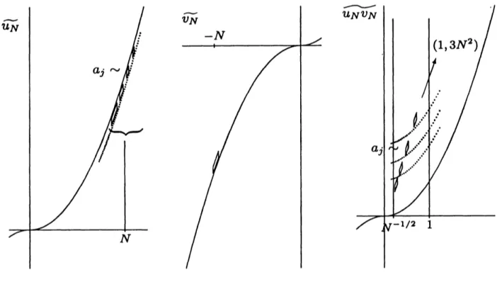
Table 1.

To

overcome

this difficulty, we have to take a real look at these counterexamples,

which

are

described in Figure 3.

For (i), $\epsilon\log N$ components of the function

$u_{N}$

are

all supported

near

the

curve

$\tau=\xi^{3}$, unlike the example given in Proposition 3. _{Thus, the stronger} $X^{-3\prime 4,1’ 2,1}$

norm

of $u_{N}$ is still given by the $\ell^{2}$

sum.

On

(i) Logarithmic divergence of the bilinear estimate in $X^{-3\prime 4,1\prime 2,1}$ (high-high-low)

(ii) Logarithmic divergence of the bilinear estimatein$X_{*}$ or $X^{-3’ 4,1\prime 2}$ (high-low-high)

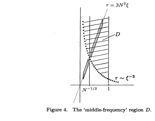
Figure 4. The ‘middle-frequency’ region $D$

.

components

are

supported in the low-frequency region between $N^{-1\prime 2}$ and 1, and also

dyadically separated with respect to $\tau-\xi^{3}$

.

Thus, the

norm

of the output amounts

to the $\ell^{1}$ sum ifwe employ the $\ell^{1}$-Besov structure in low frequency. We remark that

all the $\ell_{k}^{p}$ norms are equivalent if a function is restricted near the

curve

$\tau=\xi^{3}$ since

there is

no

summation

over

$k$ in such a case, and that the modification from $\ell_{k}^{2}$ to $\ell_{k}^{1}$

has

an

effect only when a function is supported away from the curve.

For (ii), the low-frequency function $v_{N}$ has $\epsilon\log N$ components between $0$ and

$N^{-1’ 2}$, and its $X^{-3’ 4,1’ 2}$

norm

is _{given by the} $\ell^{2}$ sum. We see that outputs of the

interaction ofthese components with $u_{N}$ fall onto almost the

same

frequencyposition

near

the curve. Therefore, the norm of the output is the $\ell^{1}$ sum,

no

matter which

structure we use in high frequency.

It is worth noting that these serious interactions come from different parts of the

low-frequency region separated by the fuzzy boundary $|\xi|\sim N^{-1’ 2}$

.

Note also that

both of them

are

supported along the line $\tau=3N^{2}\xi$

.

This suggests that

we

may

use

$X^{-3’ 4,1’ 2}$ _{in the middle frequency region}

$D:=\{(\tau, \xi)\in \mathbb{R}^{2}||\xi|<1,$ $|\tau|>|\xi|^{-3}\}$,

and use $X^{-3\prime 4,1\prime 2,1}$ in very low frequency

$\{|\xi|<1\}\backslash D$; see Figure 4. In fact, itturns

out that the high-high-low interaction can be controlled in very low frequency

even

if

we assume the stronger structure $X^{-3\prime 4,1’ 2,1}$ there, and that the high-low-high can

be still controlled under the weaker structure $X^{-3\prime 4,1’ 2}$ in middle frequency.

Our working space $X$ is defined by

where $P_{D}$ is the frequency-localizing operator to the set $D$

.

For this $X$ we

can

establish the desired bilinear estimate, Proposition 1.

4.

Local well-posedness

In addition to the bilinear estimate, the following linear estimates

are

verified.

Lemma 1. We have the following estimates

$\Vert e^{-t\partial_{x}^{3}}u_{0}\Vert_{X_{|\sim 1,1[}}+\sup_{-1\leq t\leq 1}\Vert e^{-t\partial_{x}^{3}}u_{0}\Vert_{H^{-3/4}(R)}\leq C\Vert u_{0}\Vert_{H^{-3\prime 4}(R)}$,

$\Vert\int_{0}^{t}e^{-(t-t’)\partial_{x}^{3}}F(t’)dt’\Vert_{X_{|-1,11}}+\sup_{-1\leq t\leq 1}\Vert\int_{0}^{t}e^{-(t-t’)\partial_{x}^{3}}F(t’)dt’\Vert_{H^{-3/4}(R)}$

$\leq C\Vert\langle\partial_{t}+\partial_{x}^{3}\rangle^{-1}F\Vert_{X}+\Vert\langle\partial_{t}+\partial_{x}^{3}\}^{-1}F\Vert_{Y}$

.

Proof is much easier than the bilinear estimate (see [13]). Remark that the

time-restricted

norm

plays the

same

role

as

the cutoff function in the estimates (3), (5).

FromProposition 1 and Lemma 1, we

can

iterate the equation in the space $X_{1-1,1]}\cap$

$C([-1,1];H^{-3’ 4}(\mathbb{R}))$ and obtainTheorem 1 except for theuniqueness; note thatthese

estimates only imply the uniqueness in

a

small ball of the working space.

It remains to extend the uniqueness to the whole working space. Recall that in

the

case

$s>-3/4$ , Kenig, Ponce, and Vega [11] showed the uniqueness of solutions

in $X^{s,b}$

$[-T,T]$’ essentially using the following stronger bilinear estimate: There exists

$\alpha=\alpha(s)>0$ such that

$\Vert\partial_{x}(\psi(\frac{t}{\delta})u\cdot\psi(\frac{t}{\delta})v)\Vert_{X^{e,b}}\leq C\delta^{\alpha}\Vert u\Vert_{X^{\epsilon.b}}\Vert v\Vert_{X^{\epsilon,b}}$ (9)

for any $\delta\in(0,1]$

.

If (9) is valid, then we

can

derive the uniqueness in $X_{[-T,T]}^{s,b}$ as follows. Let $u,$$v\in$

$X_{1-T,T]}^{s,b}$ be two solutions of the integral equation on

a

time interval $[-T, T]$ with the

same

initial datum $u_{0}$

.

Then, $\psi(t/\delta)u$ and $\psi(t/\delta)v$ solve the equation on $[-\delta’, \delta’]$,

where $\delta’=\min\{\delta, T\}$

.

Therefore, we have

$u(t)-v(t)= \int_{0}^{t}e^{-(t-t’)\partial_{x}^{3}}\partial_{x}[(\psi(\frac{t’}{\delta})u(t’))^{2}-(\psi(\frac{t’}{\delta})v(t’))^{2}]dt’$

on $[-\delta’, \delta’]$

.

We

see

from (5) and (9) that

$\Vert u-v\Vert_{X_{|-\delta’.\delta’|}^{\epsilon,b}}\leq C\delta^{\prime\alpha}\Vert u+v\Vert_{X_{11}^{s,b}}\Vert u-v\Vert_{X_{|-\delta’,\delta’|}^{s,b}}-\delta’,\delta’$

for $\delta’\in(0,1]$

.

Since _{$\Vert u+v\Vert_{X_{|-\delta\delta|}^{\epsilon,b}},,’\leq\Vert u||_{X_{|-T,T|}^{s,b}}+\Vert v\Vert_{X_{|\sim T,T|}^{\epsilon,b}}$},

we

can

choose $\delta$

so

the case $T>\delta’=\delta$, the uniqueness in $X_{[-T,T]}^{s,b}$ will be obtained by repeating this

procedure.

In

our

context, however, estimate like (9) is not available. One of the

reasons

for this is the criticality of the problem; in fact, the exponent $\alpha(s)$ given in (9)

tends to $0$

as

$sarrow-3/4$

.

We employ the argument of Muramatu and Taoka [16],

who considered the local well-posedness for nonlinear Schr\"odinger equations with

quadratic nonlinearities. In this argument, the following fact is essential:

$\lim_{\deltaarrow 0}\Vert u\Vert_{Z_{|-\delta,\delta l}}=0$ (10)

for $u\in z_{1-T,T]}$ with

some

$T>0$

satisfying ,$u|_{t=0}=0$, where $Z;=X\cap$

$C(\mathbb{R};H^{-3/4}(\mathbb{R}))$. For the proof of (10), we refer to [16, 13].

Let $u,$$v\in Z_{1-T,T]}$ be

as

above. Using Lemma 1 and Proposition 1, we

see

that

$\Vert u-v\Vert_{Z_{|-\delta\delta[}},,’\leq C\Vert u+v\Vert_{Z_{|-\delta\delta J}},,’\Vert u-v\Vert_{Z_{|-\delta\delta l}},,$

”

so

it suffices to make $\Vert u+v\Vert_{Z_{|-\delta\delta)}},,$

’ small. We split it between $\Vert u+v-$

$2e^{-t\partial_{x}^{3}}u_{0}\Vert_{Z_{|-\delta\delta 1}},,$

’ and $2\Vert e^{-t\partial_{x}^{3}}u_{0}\Vert_{Z_{|-\delta\delta l}},,’$

.

Then, the first

one

can be arbitrarily small

with the aid of (10), since $u+v-2e^{-t\partial_{x}^{3}}u_{0}|_{t=0}=0$

.

On the other hand, Lemma 1

bounds the second term by $C\Vert u_{0}\Vert_{H^{-3/4}}$, so we can make it small by the scaling

argument, and then obtain the uniqueness in $Z_{1-\delta’,\delta’]}$ for sufficiently small $\delta$

.

The

desired uniqueness follows after repeating it.

5. Global

well-posedness

and

the

I-method

Here, we briefly review the argument in [5], which established the global

well-posedness in $H^{s}(\mathbb{R})$ for $s>-3/10$, to see the

essence

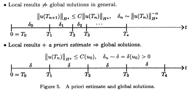
of the I-method.

In general, global well-posedness is obtained by pasting the local results. However,

the basic local result, which gives the existence time $\delta\sim\Vert u_{0}\Vert^{-\alpha}$ with

some

$\alpha>0$

and the estimate $\sup_{-\delta\leq t\leq\delta}\Vert u(t)\Vert\leq C\Vert u_{0}\Vert$, is not sufficient by itself, because in

each step, the initial datum may grow exponentially and provide the

exponentially-decaying existence time. Therefore, we need

some

a priori estimate

on

the growth

of the solution which bounds the data uniformly in each step;

see

Figure 5. For

instance, the $L^{2}$ conservation of the real-valued _$KdV$ solution together with LWP in

$L^{2}$ immediately yields GWP of (1) in $L^{2}$ in the real-valued setting.

However, when we consider negative Sobolev regularities, there is no conservation

law or a priori estimate on the $H^{s}$ norm of solutions. We now introduce

an

almost

conserved quantity which controls the time of local existence in place of the $H^{s}$

norm.

Let $N\gg 1$ _{and $s<0$}

.

_{We define $I=I_{s,N}$}

as

_{the spatial Fourier multiplier with}

the symbol $m_{s,N}(\xi)=m_{s}(|\xi|/N)$, where $m_{s}(r)$ : $\mathbb{R}_{+}arrow \mathbb{R}_{+}$ is

a

smooth monotone

function which equals 1 for $r\leq 1$ and $r^{s}$ for _{$r\geq 2$}

.

We have $C^{-1}\Vert\phi\Vert_{H^{\epsilon}}\leq$

II

$I\phi\Vert_{L^{2}}\leq$

$\bullet$ Local results $\neq$ global solutions in general.

$\Vert u(T_{n+1})\Vert_{H}$

.

$\leq C\Vert u(T_{n})\Vert_{H}.$, $\delta_{n}\sim\Vert u(T_{n})\Vert_{H}^{-\alpha}$

$\frac{1\delta_{01}\delta_{11}\delta_{2|}}{||||,T_{1}T_{2}T_{3}}$

.

.

.

$\tau_{*}^{1}|\ldots\ldots\ldots\ldots\ldots\ldots\ldots\ldots\ldots\ldots\ldots\ldots\ldots\ldots\ldots..\rangle t$ $0=T_{0}$

$\bullet$ Local results $+a$ priori $estimate\Rightarrow$ global solutions.

$\Vert u(T_{n})\Vert_{H^{s}}\leq C(u_{0})$, $\delta_{n}\sim\delta=\delta(u_{0})>0$

$||||||||\ovalbox{\tt\small REJECT}^{\backslash }|\delta|\prime t$

$0=T_{0}$ $T_{1}$ $T_{2}$ $T_{3}$ $T_{4}$

Figure 5. A priori estimate and global solutions.

Lemma 2 ([5]). Let

_$s>-3/4$

.

Then, there exists

$b>12$

such that

_for

any

$u_{0}\in H_{f}^{s}$

a

solution $u(t)\in C([-\delta, \delta];H^{S})$ to (1) exists

on

$[-\delta, \delta]$ with $\delta\geq c\Vert Iu_{0}\Vert_{L^{2}}^{\sim\alpha}$

and

_satisfies

$\Vert Iu\Vert_{X_{|-\delta,\delta 1}^{0,b}}\leq C\Vert Iu_{0}\Vert_{L^{2}}$

.

Here $c,$ $C$, and $\alpha$

are some

positive constants

independent

_of

$N$

.

Another important feature of the operator $I$ is almost _$consen$)$ation$ of $||Iu(t)||_{L^{2}}$

.

Lemma 3 ([5]). Let $u(t)$ be a real-valued solution to the $KdV$ equation on the time

interwal $[-\delta, \delta]$

.

Then,

for

any $\epsilon>0$ and $b>1/2$ there exists $C>0$ independent

of

$N$ such that

$\Vert Iu(t)\Vert_{L^{2}}^{2}\leq\Vert Iu(0)\Vert_{L^{2}}^{2}+CN^{-3/4+\epsilon}\Vert Iu\Vert_{X_{|-\delta,\delta l}^{0,b}}^{3}$

$for-\delta\leq t\leq\delta$

.

It follows from Lemmas 2 and 3 that if $s>-3/4$ and the real-valued initial datum

$u_{0}$ satisfies $\Vert Iu_{0}\Vert_{L^{2}}\leq 1$, then we can iterate the local theory $O(N^{3\prime 4-\epsilon})$ times until

the norm $\Vert Iu(t)\Vert_{L^{2}}$ becomes greater than 2. We thus obtain solutions at least up to

$t=O(N^{3/4-\epsilon})$ from such initial data.

For general data, we utilize the scaling argument. If the datum satisfies

$\Vert Iu(0)\Vert_{L^{2}}\leq M$, then

we

first rescale it so that

$\Vert Iu^{\lambda}(0)\Vert_{L^{2}}\leq CM\lambda^{-3’ 2-s}N^{-s}=1$ $\Leftrightarrow$ $\lambda\sim(MN^{-s})^{2\prime(3+2s)}$,

and solve the equation from the rescaled datum. Rescaling back to the original one,

we

obtain

a

solution up to the time $t=O(\lambda^{-3}N^{3\prime 4-\epsilon})$

.

Therefore,

we

can

solve

the equation on an arbitrarily large time interval, by taking $N$ sufficiently large,

if $\lim_{Narrow\infty}\lambda^{-3}N^{3\prime 4-\epsilon}=\infty$

.

This condition is equivalent to

$-6s’(3+2s)<34$

, or

To show the global results in $H^{-3\prime 4}$, we have to add

some

correction terms to the

almost conserved quantity $\Vert Iu(t)\Vert_{L^{2}}$ and improve the decay with respect to $N$ in

Lemma

3. See

[6] for details.

6. Remark

Recently, Guo [9] obtained the same well-posedness results independently. The

function space in the work of Guo [9] is identical with

our

space in high frequency.

The only difference is in low frequency $\{|\xi I \leq 1\}$; the space in [9] has the maximal

function norm $\Vert P_{0}u\Vert_{L_{x}^{2}(L_{t}^{\infty})}$, while

our

space is defined by

$\Vert P_{D}u\Vert_{X^{0,1/2}}+\Vert P_{0}(1-P_{D})u\Vert_{X^{0,1/2,1}}$ $(+\Vert P_{0}u\Vert_{L_{t}^{\infty}(L_{x}^{2})})$.

These structures share

some common

properties; for instance, both

are

weaker than

$X^{-3’ 4,1\prime 2,1}$ for the high frequency _{part and stronger than $C(H^{-3’ 4})$}

.

_{However, there}

is no inclusion relation between two spaces.

On the other hand, in contrast to the space in [9] defined on the physical space $\mathbb{R}_{t,x}^{2}$

in low frequency, we define our space $X$ totally on the Fourier space $\mathbb{R}_{\tau,\xi}^{2}$ similarly

to the standard $X^{s,b}$

.

This feature of our space allows us to define an auxiliary space for the estimate

of nonlinearity simply as $\langle\partial_{t}+\partial_{x}^{3}\rangle X$, and completely separate the estimate for the

Duhamel term of the integral equation, like (4), into the linear Duhamel estimate,

like (5), and the bilinear estimate, like (6). The

same

reduction would be nontrivial

for function spaces including the

norm on

the physical space. Moreover, the space

in [9] should be considered in the time-restricted form, i.e. with a temporal bump

function, because the $L_{t}^{2}(L_{x}^{\infty})$ maximal function estimate does not hold globally in

time. Such restriction in time is not needed for

our

space in proving the bilinear

estimate.

We should also make a crucial remark that

our

space $X$ has the monotonicity in

frequency, namely, $|\tilde{u}|\leq|\tilde{v}|$ implies $\Vert u\Vert_{X}\leq\Vert v\Vert_{X}$, which does not hold in the space

defined on the physical space $\mathbb{R}_{t,x}^{2}$

.

We actually

use

this property in the proof of

required linear estimates Lemma 1. Such structure is also compatible with the

I-method and admits the identical proof for the global well-posedness

as

the previous

one

([6]) working

on

the standard $X^{s,b}$

.

Acknowledgment

The author would like to express his great appreciation to Professor Yoshio

Tsutsumi for encouraging him to address this issue and giving him a number of

valuable advices. He also offers his thanks to Professor Zihua Guo for valuable

discussion, and also to Professor Hideo Takaoka for informing him of the work of

References

[1] J.L. Bona and F.B. Weissler, Pole dynamics

_of

interacting solitons and blomup

_of

complex-vdued solutions

_of

KdV, Nonlinearity 22 (2009), 311-349.

[2] J. Bourgain, Fourier

_transform

restriction phenomena

_for

certain lattice subsets and

applications to nonlinear evolution equations, I, $Schr\delta dinger$ equations, Geom. Funct.

Anal. 3 (1993), 107-156.

[3] J. Bourgain, Fourier

transform

restriction phenomena

_for

certain lattice subsets and applications to nonlinear evolution equations, $\Pi$, Geom. Funct. Anal. 3 (1993),

209-262.

[4] M. Christ, J. Colliander, and T. Tao, Asymptotics, frequency moddation, and low

regularity ill-posedness

_for

canonical defocusing equations, Amer. J. Math. 125 (2003),

1235-1293.

[5] J. Colliander, M. Keel, G. Staffilani, H. Takaoka, and T. Tao, Globalwell-posedness

_for

KdV in Sobolev spaces

_of

negative index, Electron. J. Differential Equations 2001, No.

26, 1-7.

[6] J. Colliander, M. Keel, G. Staffilani, H. Takaoka, and T. Tao, Sharp global

well-posedness

_for

KdV and

_modified

KdV on $\mathbb{R}$ and I, J. Amer. Math. Soc. 16 (2003),

705-749.

[7] D.G. Crighton, Applications

_of

KdV, Proceedingsof the intemationalsymposium KdV

95” (Amsterdam, 1995); Acta Appl. Math. 39 (1995), 39-67.

[8] J. Ginibre, Y. Tsutsumi, and G. Velo, On the Cauchy problem

_for

the Zakharov system,

J. Fhnct. Anal. 151 (1997), 384-436.

[9] Z. Guo, Global well-posedness

_of

Korteweg-de Vries equation in $H^{-3’ 4}(\mathbb{R})$, J. Math.

Pures Appl. 91 (2009), 583-597.

[10] C.E. Kenig, G. Ponce, and L. Vega, Well-posedness and scattering results

_for

the gen-eralized Korteweg-de Vries equation via the contraction principle, Comm. Pure Appl.

Math. 46 (1993), 527-620.

[11] C.E. Kenig, G. Ponce, and L. Vega, A bilinear estimate with applications to the KdV

equation, J. Amer. Math. Soc. 9 (1996), 573-603.

[12] C.E. Kenig, G. Ponce, and L. Vega, On the ill-posedness

_of

some canonical dispersive

equations, Duke Math. J. 106 (2001), 617-633.

[13] N. Kishimoto, Well-posedness

_of

the Cauchy problem

_for

the Korteweg-de Vries equation

at the $C7\dot{n}tical$ regularity, Differential Integral Equations 22 (2009), 447-464.

[14] N. Kishimoto, Counterexamples to bilinear estimates

_for

the Korteweg-de Vries equation

in the Besov-type Bourgain space, to appear in Funkcial. Ekvac.

[15$|$ D.J. Korteweg and G. de Vries, On the change

of

form

of

long waves advancing in a

rectangular canal, and on a new type

_of

long $stationa\eta$ waves, Philos. Mag. 39 (1895),

422-443.

[16] T. Muramatu and S. Taoka, The initial value problem

_for

the 1-D semilinear

Schrodinger equation in Besov spaces, J. Math. Soc. Japan 56 (2004), $85\succ 888$

.

[17] K. Nakanishi, H. Takaoka, and Y. Tsutsumi, Counterexamples to bilinear estimates

related vJith the KdV equation and the nonlinear Schrodinger equation, Methods Appl.

Anal. 8 (2001), 569-578.

[18] D. Tataru, Local and globd results

_for

wave maps, I, Comm. Partial Differential Equa-tions 23 (1998), 1781-1793.