On the design and analysis of evolutionary algorithms (Algorithm Engineering as a New Paradigm)

On

the design and analysis

of

evolutionary

algorithms*

Ingo Wegener

FB Informatik, $\mathrm{L}\mathrm{S}2$, Univ. Dortmund

44221 Dortmund, Germany

wegener@ls2.$\mathrm{c}\mathrm{s}.\mathrm{u}\mathrm{n}\mathrm{i}$-dortmund.de

Abstract: Evolutionary algorithms are problem-independent randomized

search heuristics. It is discussed when it is useful to work with such algorithms and

it is argued why these search heuristics should be analyzed just as all other deterministic

and randomized algorithms. Such an approach is startedby analyzing asimple evolutionary

algorithm on linear functions, quadratic functions, unimodal functions, and its behavior on

plateaus of constant fitness. Furthermore, it is investigated what can be gained and lost by

a dynamic variant of this algorithm. Finally, it is proved that crossover can decrease the

run time ofevolutionary algorithms significantly.

Keywords: evolutionary algorithms, analysis of algorithms, crossover.

1

Introduction

The historyofevolutionaryalgorithms datesback

to the sixties (see Fogel (1985), Goldberg (1989),

Holland (1975), or Schwefel (1995), the

hand-book edited by B\"ack, Fogel, and Michalewicz

(1997) presents all developments). It is aclassof problem-independent randomized search

heuris-tics used for optimization, adaptation, learning,

and some other aims. Here we focus on

opti-mization. Randomization is also a major tool

for problem-independent algorithms (see

Mot-wani and Raghavan (1995)$)$. Nevertheless, there

is almost no contact between people working

on evolutionary algorithms and people

work-ing on classical randomized optimization

algo-rithms. The reasons are certain

misunderstand-ings. Many people doubt the need for problem-independent search heuristics and argue that

problem-dependent algorithms have to better,

since they are based on problem-specific

knowl-edge. We discuss these aspects in Section 2.

There we present some realistic scenarios where

onehas towork with problem-independent search

heuristics.

The classical research on efficient algorithms

combines the design and the analysis of

algo-*Thisworkwassupported bythe Deutsche Forschungs-gemeinschaft (DFG) aspartofthe Collaborative Research Center ($‘ \mathrm{C}\mathrm{o}\mathrm{m}\mathrm{p}\mathrm{u}\mathrm{t}\mathrm{a}\mathrm{t}\mathrm{i}\mathrm{o}\mathrm{n}\mathrm{a}\mathrm{l}$Intelligence” (SFB 531).

rithms. There are only few analytical results

on evolutionary algorithms comparable to the analytical results on the classical algorithms.

The analysisofa problem-independent algorithm working on aspecific problem is typically harder

than the analysis of problem-specific algorithms

which often are designed to support the analysis.

We discuss $\mathrm{i}\dot{\mathrm{n}}$

Section3 the limited value of often

discussed statements on evolutionary algorithms

and argue whythe analysis ofevolutionary

algo-rithms should be performed in the same way as

the analysis of all other types of algorithms. In

the rest of the paper we present shortly results

which have been obtained this way.

In Section 4, we introduce the (I+I)EA, the

perhaps simplest evolutionary algorithm which

is in many situations surprisingly successful.

The next three sections consider the analysis of

the $(1+1)\mathrm{E}\mathrm{A}$ on pseudo-boolean functions $f$ :

$\{0,1\}^{n}arrow \mathbb{R}$ in order to prove or to disprove well

accepted conjectures. In Section 5, it is shown

that the (I+I)EA optimizes linear functions

ef-ficiently. However, statements on the efficiency

on classes of functions are difficult. In Section

6, two conjectures are disproved namely the

con-jectures that the (I+I)EA is efficient for all

uni-modal functions and for all functions of small

de-gree. In Section 7, the behavior of the $(1+1)\mathrm{E}\mathrm{A}$

and one of its variant on plateausof constant

mutation probability $1/n$. In Section 8, we

ana-lyze a dynamic variant of the $(1+1)\mathrm{E}\mathrm{A}$ working

with alternatingmutation probabilities.

The$(1+1)\mathrm{E}\mathrm{A}$usesonly nlutation andselection.

Many people believe that crossover is a

funda-mental operation. Nevertheless, this was proved

by experiments only. In Section 9, we present

the first proof thatcrossover can decrease the

ex-pected run time for a specific function from

su-perpolynomial to polynomial.

The main purpose ofthis paper is to convince

$\mathrm{r}\mathrm{e}\mathrm{s}\mathrm{e}\mathrm{a}\mathrm{r}\mathrm{c}\mathrm{h}\dot{\mathrm{e}}\mathrm{r}\mathrm{S}$

that evolutionary $\mathrm{a}\mathrm{l}\mathrm{g}’ \mathrm{o}\mathrm{r}\mathrm{i}\mathrm{t}\mathrm{h}\mathrm{m}\mathrm{S}$ are a

generic part of the research area of efficient al-gorithms.

2

Scenarios for

general

random-ized search heuristics

First, we have to define the notion of

random-ized search heuristics. For some state space $S$,

we look for heuristics to find efficiently good or

even op.timal$\dot{\mathrm{p}}\mathrm{o}\mathrm{i}\mathrm{n}\mathrm{t}_{\mathrm{S}\mathrm{f}\mathrm{o}}\mathrm{r}..\xi \mathrm{u}\mathrm{n}\mathrm{c}\mathrm{t}\mathrm{i}_{0}\mathrm{n}\mathrm{s}f$: $Sarrow \mathbb{R}$. The

mainhandicap ofthe search is thatthealgorithm

does not “$\mathrm{k}\mathrm{n}\mathrm{o}\mathrm{W}$”

$.$

f.in.

advance. It can sample $f$,

i.e., itcan choose searchpoints$x$ from$S$andthen

evaluate $f(X\backslash )$. The furthersearch canbe directed

by the partial knowledge

_about.

$f$

obtain.e

$\mathrm{d}$ from

previous sampling.

Definition 1 Randomized search $heurist\dot{i}.c$

for

real-valued

_functions

on $S$.

The

_first

search point $x_{1}$ is chosen according to

a $probab\dot{i}l_{\dot{i}}ty$ distribution on $S$ specified by the

heuristic. $T\dot{h}$en

$f(x_{1})$

for

the actual $f$ is

eval-uated. The search point $x_{t}$ is chosen

accord-ing to a probability distribution which is

speci-fied

by the heuristic and which may depend on

$(x_{1}, f(x_{1}),$$\ldots$,$x_{t-1},$$f(x_{t1}-))$. Then$f(x_{t})$ is

eval-uated. The process is iterated until a stopping criterion is

_fulfilled.

This definition captures all randomized search

heuristics. If an algorithm starts with $n$

ran-domly chosen search points, this is captured

by Definition 1, since the search points $x_{i}$,

$2\leq\dot{i}\leq n$, can be chosen independently from $(x_{1}, f(x_{1}),$

$\ldots,$$Xi-1,$$f(X\mathrm{i}-1))$. The consideration

of so-calledpopulations is spaceefficient and

pre-scribes that the further search process is

inde-pendent from allsampledsearch pointswhich are

not in the actual population. Figure 1 illustrates the $\acute{\mathrm{m}}$

ain differences between the classical

opti-mizationscenario and the so-called black-box

op-timization scenario which assumes that the

func-tion $f$ to be optimized is hidden in _sonle

black-box.

classical optimization

black box optimization

Figure 1: Optimization scenarios.

Thedesignof problem-specific algorithms is

in-fluenced by the results of the analysis of the

analytical results and the experimental

experi-enceabouta problem-independent algorithm on a

specific problem should have not too much

influ-enceon thedesignofthisalgorithm as a

problem-independent one. Only results and experiments

on many different problems should have such an

influence. Otherwise, the algorithm may turn

into a problem-specific one. The question is

why weneed problem-independent algorithms. If

we know a problem, analyze it and use all our

knowledge todesigna problem-specificalgorithm,

thisshould be better than a problem-independent

algorithm. Nobody should doubt this.

How-ever, there are at least two situations or scenar-ios where one needs problem-independent

algo-rithms.

Scenario 1 A problem has to be solved quickly

on not too many instances and there are not

enough resources (time, money, $and/or$

knowl-edge) to design a problem-specific algorithm.

Thisscenariois realistic in applications. There

are not so many experts in designing algorithms that all optimization problems in applicationscan

be attacked by them.

Scenario 2 The

_function

$f$ : $Sarrow \mathbb{R}$ is not

‘known” and one can only $\dot{‘}{}^{t}s$

ample” $f$.

Ifone likesto optimizeacomplicatedtechnical

system by fixing some free parameters, it

hap-pens that the technical system is so complicated

that its input-output behavior cannot be

com-puted and only experiments improve the

knowl-edge about the system.

Inblack-box optimization the cost is measured

by the number of search points which are

sam-pled.

3

How

to

analyze evolutionary

algorithms

First, we introduce the essential modules of EAs

(evolutionary algorithms):

-Selection is used to decide which search

points will be forgotten (the others are the

members of the actual population called

gen-eration) and it is also used to decide which

“individuals” ofthe “currentpopulation” are

chosen as “parents”.

-Mutation and crossover produce new

indi-viduals called “children” from the parents.

Mutation works onone parent and produces

usually one child while crossover works on

at least two parents (most often exactly two parents) and produces a certain number of

children.

Evolutionary algorithms are designed as

ro-bust search heuristics with the hope that they

are quite efficient on many problems of

differ-ent type. However, often exaggerated statements

like “an evolutionary algorithm is better than all

other algorithms on the average of all problems”

have been used. The NFL theorem of Wolpert

andMacready (1997) shows that such statements

are wrong and it is necessary to analyze

evolu-tionary algorithms more carefully. Too general

statements tend to be wrong. This is also the

case with the building block hypothesis. Mitchell,

Forrest, and Holland (1992) have presented the

so-called royal-road functions whereevolutionary

algorithms with crossover should have big

ad-vantages if the building block hypothesis holds.

Later they have admitted that a simple

evolu-tionaryalgorithm outperforms genetic$\mathrm{a}\mathrm{l}\mathrm{g}\mathrm{o}\mathrm{r}\mathrm{i}\mathrm{t}\dot{\mathrm{h}}\mathrm{m}\mathrm{S}$

which rely on crossover (Mitchell, Holland, and Forrest (1994)$)$. The often cited schema theo-remis acorrect but simpleresult onthe behavior

within one step. Other one step measures like

the quality gainand the progress rate arewell

an-alyzed. The results describe the microscopic be-havior, but inmany situations thisimpliesalmost

nothing for the macroscopic behavior. Finally, evolutionary algorithms are analyzed as

dynam-ical systems and therefore implicitly under the

assumption of

an.

_infi.nite

population. Then the

difference between finite andinfinite populations

has to be investigated carefully. Rabani,

Rabi-novich, and Sinclair (1995) have started such an

approach.

We have chosen another $\mathrm{p}\mathrm{o}\mathrm{i}\mathrm{n}\mathrm{t}\backslash$of view. A

ran-domized search heuristic isnothingbuta

random-ized algorithm and shouldbe analyzed like a

ran-domized algorithm with one distinction. Since $f$

is assumed to beunknown,

on..e

neverknowswhen

theoptimum is reached. Hence, we consider

evo-lutionary algorithms without stopping criterion

and investigate random variables $x_{f}$ measuring

the first point of time where on$f$ something nice

of an optimal search point and we consider the

maximization of $f$

.

Our interest (motivated by

the requirements ofapplications) is the behavior

within reasonable time bounds and not the limit

behavior. Moreover, we are interested in the

be-havior for typical functions (typical instances for

classicalalgorithms). Thisleads to bounds on the

best and worst case behavior on classes of

func-tions (problems for classical algorithms). Such

resultscan be used to compare different

random-ized search heuristics.

The obvious problem is to estimate the

ex-pected search time $E(X_{f})$

.

This expected value

can be exponentially large, although the event

“_{$x_{f}\leq t(n)$}” _{for small $t(n)$ has} a _probability

which isnot toosmall. Such a result is ofspecial

interest, sincewehavethe multi-startoption, i.e.,

many independent runs of the algorithm can be

performed in parallel.

4

The

simple

$(1+1)\mathrm{E}\mathrm{A}$

Algorithm 1 $(l+l)EA$

- choose $x\in\{0,1\}^{n}$ randomly,

- let $x’$ be the result

of

a mutation

of

$x,\dot{i}.e.$,

the bits $x_{i}’$ are generated independently and $x_{i}’=\overline{x}_{i}$ with themutation probability$1/n$ and

$x_{i}’=x_{i}$ otherwise, . ’

- _$x$ is replaced with $x’$

iff

$f(x’)\geq f(x)$,

- the last two steps are iterated.

The notation $(1+1)\mathrm{E}\mathrm{A}$ means that the

popu-lation size is 1, the current search point creates

one child by mutation and the child replaces its

parent iff it is not worse than its parent. One

can easily design algorithms with larger

popula-tions. However,selection has thetendencyto

cre-ate populations with a smalldiversity. Hence,one

canprove inmany casesthat$p$independent runs

of the (I+I)EA outperform an evolutionary

al-gorithm with population size$p$. This will not be

discussed here in detail, but we sometimes

men-tion the behavior of multi-start variants.

5

The

$(1+1)\mathrm{E}\mathrm{A}$

on

linear

func-tions

Definition 2 A

_function

$f$ : $\{0,1\}^{n}arrow \mathbb{R}$ is

called linear $\dot{i}ff(x_{1,\ldots,n}x)=w_{0}+w_{1}x_{1}+\cdots+$

$w_{n}x_{n}$

.

For theanalysisofthe $(1+1)\mathrm{E}\mathrm{A}$ onlinear

func-tions we can

assume

without loss of generality

that $w_{0}=0$ and $w_{1}\geq\cdots\geq w_{n}>0$. Droste,

Jansen, andWegener (1998a) haveproved the fol-lowing result which has been an open conjecture for several years.

Theorem 1 The expected run time

_of

the

$(l+l)EA$ with non-zero linear weights equals

$\ominus(n\log n)$

.

In this survey article weonlylist the main ideas

of the proofs. The lower bound followseasily with

the Chernoff’s bound, showing that the initial

point has alarge Hamming distance to the

opti-mum, and the coupon collector’s theorem,

prov-inga bound onthe time untilthe bits different to

the bits ofthe optimumhave tried to flip at least

once.

The simpliest case where $w_{1}=\cdots=w_{n}=1$

hasbeen solvedbyM\"uhlenbein(1992). A general

upper bound of$O(n^{2})$ canbeobtainedeasily. Let

$A_{i}=\{X|w1+\cdots+w_{i}\leq f(x)<w_{1}+\cdots+wi+1\}$.

Then it is easy to see that for the Hamming dis-tance $H$ and $\dot{i}<n$

$\forall x\in A_{i}\exists y\in A_{i+1}\cup\cdots\cup A_{n}$ : $H(x, y)=1$.

Hence, the expected time to leave $A_{i}$ is bounded

above by $e\cdot n$ leading to the upper bound $e\cdot n^{2}$.

The proof method for the upper bound of

The-orem 1 is best explained for the special case of

the binary value function BV defined by

$\mathrm{B}\mathrm{V}_{n}(x)=x_{1}2^{n-1}+x_{2}2^{n-2}+\cdots+x_{n-1}2+x_{n}$.

The crucial fact is thatsteps increasing the

Ham-ming distanceto the optimal point 1n can be

ac-cepted. Theleftmost flipping bit decideswhether

the child is accepted ($0arrow 1$ is accepted, $1arrow 0$

is rejected). There may be many 1-bits to the

successful steps ($x’$ replaces $x$ and $x’\neq x$) and

unsuccessful steps.

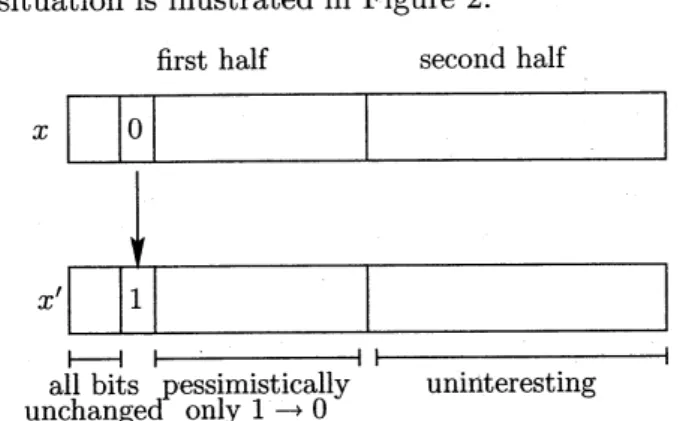
We define a Markoff process which is provably

slower than the $(1+1)\mathrm{E}\mathrm{A}$ and we measure the

progress with respect to a potential function. The

situation is illustrated in Figure 2.

firqt half $.\mathrm{q}\mathrm{e}.\mathrm{r}\cdot.0\eta \mathrm{d}$half

We need a tedious case inspectionto control the

progress with respect to this pontential

func-tion and we also have proved ageneralization of

Wald’sidentity.

6

The

$(1+1)\mathrm{E}\mathrm{A}$

on

unimodal

functions and

quadratic

func-tions

Figure 2: A successful mutation step for $\mathrm{B}\mathrm{V}_{n}$.

The potential function counts the number of

ones in the first half. For $\mathrm{B}\mathrm{V}_{n}$, the last half has

no influence onthedecision whether astepis

suc-cessful–aslongas some bit in thefirst halfflips.

A step is successful iff the first flipping bit is a

$0$. With respect to the potentialfunction we

pes-simistically assume that all other flipping bits in

the first half flip from $0$ to 1. We look for an

upper bound on the number of successful steps

$.\mathrm{u}\mathrm{n}\mathrm{t}\mathrm{i}\mathrm{l}|$ the $\mathrm{n}\mathrm{u}\mathrm{m}$

. ber

$.0..\mathrm{f}$ones in

th.

$\mathrm{e}\mathrm{f}\mathrm{i}\mathrm{r}\mathrm{S}\mathrm{t}|$

h.alf

has

in-creased from $\dot{i}$ to a larger value. The number of

ones is by our assumption a random walk on $\mathbb{Z}$

(in order to $\mathrm{o}\mathrm{b}\mathrm{t}\mathrm{a}\mathrm{i}\dot{\mathrm{n}}$

a homogeneous random walk,

we allow negative numbers). The difference

be-tween two consecutivepoints oftime is described

by a random variable $Y$ where (by our

assupm-tion) $Y\leq 1$ and (as one can prove) $E(Y) \geq\frac{1}{2}$

(here it is essential to consider only one half of the string). By Wald’s identity, the number of

successful steps until the number ofones has

in-creased is bounded by 2. Ifthe first half consists

ofones only, the same analysis works for the

sec-ond half, if one takes into account that no bit

from the first half flips in successful steps. The

probability of a successful stepis for strings with

$\dot{i}$ ones in the corresponding half bounded below

by$e^{-1}\cdot(n-\dot{i})/n$ leading to the proposed bound.

The situation of general linear functions is

much more difficult. However, a very simple

po-tential function canbe used namely

$v(x).–2\cdot(_{X_{1}}+\cdots+x_{n//+}2)+(x_{n}21+\cdots+xn)$.

The following conjectures had a great influence

in the discussion on evolutionary algorithms.

First, we introduce the notion of unimodal and

quadratic functions.

Definition 3 $\dot{i}$) A

function

$f$ : $\{0,1\}^{n}arrow \mathbb{R}$

is called unimodal $\dot{i}f$ it has a unique global

optimum and all other search points have a

Hamming neighbor with a larger

_fitness.

$\dot{i}\dot{i})$ A

function

_$f$ : $\{0,1\}^{n}$ $arrow$ $\mathbb{R}$ is called

quadratic

_if

$f(X_{1}, \ldots, X_{n})=w0$ $+ \sum_{1}\leq i<j\leq niwj+\sum_{1\leq}i\leq nwiXix_{i^{X}j}$

.

The conjectures claim that the (I+I)EA is

ef-ficient on all unimodal andon all quadratic

func-tions. Both conjectures are wrong proving that

statements that evolutionary algorithms are

ef-ficient on not very “simple” classes of functions

are in general not true. The class of unimodal

functions includes path functions.

Definition 4 A path$p$ starting at $a\in\{0,1\}^{n}$ is

defined

by a sequence

_of

points $p=(p_{0}, \ldots,p_{m})$

where $p_{0}=a$ and $H(p_{i},p_{i}+1)=1$

.

A

function

$f$ : $\{\dot{0}, 1\}^{n}arrow \mathbb{R}$ is a path$f\dot{u}nct_{\dot{i}}on$ with respect to

the path $p$

if

$f(p_{i+1})>f(p_{i})$

for

$0\leq i\leq m-1$

and $f(b)<f(a)$

_for

all $b$ outside the path.

Path functions where the fitness outside the

path is defined in such a way that the $(1+1)\mathrm{E}\mathrm{A}$

reaches the pathwith high probability at the

be-ginning of the path may lead to the conjecture

that the (I+I)EA “has to follow” the path which

would take an expected time of $(kn)$. Horn,

Goldberg, and Deb (1994) have defined

expo-nentially long paths leading to unimodal

func-tions. However, Rudolph (1997) has shown that

where only a few bits flip (here three bits) and

where the progress on the path is exponentially

large. The so-called long-path functions are

op-timized bythe (I+I)EA in expected $\mathrm{t}\mathrm{i}\mathrm{m}\mathrm{e}\ominus(n^{3})$.

Rudolph (1997) hasdefined otherlong-path

func-tions such that for all $\dot{i}\leq n^{1/2}$ each point

$p_{j}$

on the path has only one successor on the path

with Hamming distance $i$, namely

$p_{i+j}$. Hence,

shortcuts are only possible by flipping $\Omega(n^{1/2})$

bits simultaneously, an event with an

exponen-$\mathrm{t}\mathrm{i}\mathrm{a}\}\mathrm{l}\mathrm{y}$small probability. Droste, Jansen, and

We-gener (1998b) have defined a unimodal function

basedonthislong pathand have provedthat the

(I+I)EA needs an expected time$\mathrm{o}\mathrm{f}\ominus(n^{3/2n^{1/}}2)2$

for this function. Additionally, it can be shown

that multi-start variants will not lead to

subex-ponential run times.

Theorem 2 There areunimodal

_functions

where

the expected run time

_of

the $(l+l)EA$ is

_of

size

$\ominus(n^{3/2n}2)1/2$.

Wegener and Witt (2000) have analyzed the

behavior of the (I+I)EA on quadratic functions.

In contrast to the class of linear functions, it is

not possible to assume without loss ofgenerality

that all weights are non-negative. The trick to replace $x_{i}$ by $\overline{x}_{i}=1-x_{i}$ does not work, since

$w_{ij}x_{i}\dot{x}_{j}$ leads by this replacement to a new term

$w_{ij}x_{j}$ which can make the weight of$x_{j}$ negative.

In $\mathrm{p}\mathrm{a}\mathrm{r}\mathrm{t}\mathrm{i}\wedge \mathrm{c}\mathrm{u}\mathrm{l}\mathrm{a}\mathrm{r}$, there are

non-u.nimodal

$\mathrm{q}\mathrm{u}\mathrm{a}\mathrm{d}\mathrm{r}\grave{\mathrm{a}}\mathrm{t}\mathrm{i}_{\mathrm{C}}$

functions essentially depending on all variables.

With the methods of the $O(n^{2})$ bound for linear

functions one obtains the following result.

Theorem 3 Let $f$ : $\{0,1\}^{n}arrow \mathbb{R}$ be a quadratic

function

without negative weights and with $N$

non-zero weights. Then the expected run time

_of

the $(\mathit{1}+. \mathit{1}..)EA-$

is.bounded

by $O(Nn^{2})$.

There is another interesting special case

namely the case of squares of linear functions,

i.e., quadratic functions which can be writtenas

$f(x)=g(x)^{2}$ _where $g(x)=w\mathrm{o}+w_{1}x_{1}+\cdots+wnx_{n}$.

Again we can assume without loss of generality

that $w_{1}\geq\cdots\geq w_{n}>0$. The case $w_{0}\geq 0$ is

not different from the case of linear functions.

However, the case $w_{0}<0$ is interesting. If

$w_{1}=\cdots=w_{n}=1$ and $w_{0}=-(n/2-1/3)$, the

(I+I)EA finds one of thelocal optima$0^{n}$ and 1n

quickly. Sitting at thesuboptimal point $0^{n}$ it has

towait for a simultaneous flipping ofall bits

lead-ing to an expected run time $\mathrm{o}\mathrm{f}\ominus(n^{n})$. However,

the probability of reaching 1n within $O(n\log n)$

steps is at least $1/2-\in$ and multi-start _variants

are very efficiellt. This result can be generalized.

Theorem 4 The expected run time

_of

the

$(l+l)EA$ on some squares

_of

linear

_functions

equals $\ominus(n^{n})$. The success probability

for

each

square

_of

a linear

_function

within $O(n^{2})$ steps is

bounded below by $1/8-o(1)$ .

Finally, Wegener and Witt (2000) present a

very difficult quadratic function. The function

$\mathrm{T}\mathrm{R}.\mathrm{A}\mathrm{P}_{n}(x_{1}, \ldots, Xn.)=$ $-(x_{1}+\cdots+x_{n})$

$+(n+1)X_{1n}*\cdots*x$

has degree $n$ and is very difficult. The fitness

function gives hints to go to $0^{n}$. However, 1n is

the global optimum. Using a reduction due to

Rosenberg (1975) $\mathrm{T}\mathrm{R}\mathrm{A}\mathrm{P}_{n}$ is reduced to

$\mathrm{T}\mathrm{R}\mathrm{A}\mathrm{P}_{n}^{*}(x_{1,\ldots\overline{\iota}}, x_{?})$ $=$

$- \sum_{\leq 1\leq in}Xi+(n+1)X_{1}x_{22}n-$

$-(n+1)1 \leq i\sum_{\leq 2n-2}(_{X}n-iXn+i-1$

$+x_{n+i}(3-2Xn-i-2X_{n}+i\neg^{1}))$,

aquadratic function with almost thesame prop-erties as $\mathrm{T}\mathrm{R}\mathrm{A}\mathrm{P}_{n}$. Nevertheless, the analysis of

the (I+I)EA on $\mathrm{T}\mathrm{R}\mathrm{A}\mathrm{P}_{n}^{*}$ is more involved than on $\mathrm{T}\mathrm{R}\mathrm{A}\mathrm{P}_{n}$.

Theorem 5 With probability 1 $-2^{-\Omega(n)}$, _the

$(l+l)EA$ needs $2^{\Omega(n\mathrm{l})}\mathrm{o}\mathrm{g}n$

steps on the quadratic

function

$TRA$

. $P_{n}^{*}$.

7

Evolutionary

algorithms

on

plateaus

of

constant fitness

Definition 5 A plateau

_for

$f$ : $\{0,1\}^{n}arrow \mathbb{R}$ is

a set $P\subseteq\{0,1\}^{n}$ such that $f(a)=f(b)$

for

all

$a,$$b\in P$ and there is path

from

$a$ to $b$ inside _$P$.

As longas anevolutionary algorithmonlyfinds

searchpointsfrom a plateau, it gets no hints how

to direct the search. The $(1 +1)\mathrm{E}\mathrm{A}$ searches

blindly on the plateau and accepts each string.

Wearediscussingplateaus whichareshort paths.

Is itpossiblefor the (I+I)EA toreach the (

of such a plateau efficiently? To be more precise,

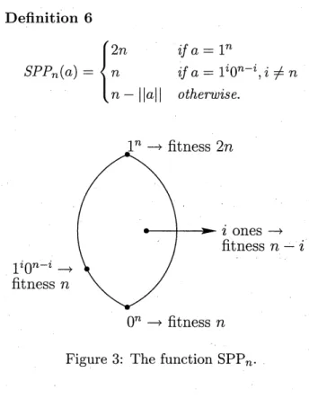
JansenandWegener(2000) have definedthe

func-tion $\mathrm{S}\mathrm{P}\mathrm{P}_{n}$ (short path as plateau), see Figure 3.

We define $||a||=a_{1}+\cdots+a_{n}$. Definition 6 $SPP_{n}(a)=\{$ $2n$

if

$a=1^{n}$ $n$ $\dot{i}fa=1^{i}0^{n-i},$$i\neq n$ $n-||a||$ otherwise.

Figure 3: The function $\mathrm{S}\mathrm{P}\mathrm{P}_{n}$.

.

Theorem 6 The expected run time

_of

the

$(1+1)EA$ on $\mathrm{S}\mathrm{P}\mathrm{P}_{n}$ is bounded by $O(n^{3})$ and the

successprobability

_for

$n^{4}$ steps is $1-2^{-\Omega(n}$).

It is easy to see that the (I+I)EA reaches the

plateau with high probability close to $0^{n}$ and is

far away from the “golden point” $1^{n}$. Then only

points from the plateau or 1n are accepted. The

$(1+1)\mathrm{E}\mathrm{A}$ makes a random walk on the plateau

like on a bounded interval of Z. A fraction of

$\ominus(1/n)$ ofthe steps is successful, since thesesteps

find another point on the plateau. The random

walk is almost symmetric (we cannot jump

“be-hind” $0^{n}$ or $1^{n}$). Now we can use results on the

gambler’s ruin problem to prove that the success

probability within $cn^{2}$ steps, _$c$ large enough, is

bounded below by a positive constant. This leads

to the bounds of Theorem 6.

For $\mathrm{S}\mathrm{P}\mathrm{P}_{n}$, it is essential to investigate the

plateau. Letthe (I+I)*EA be thevariant which

accepts $x’$ only if $f(x’)>f(x)$. The (I+I)*EA

also finds the plateau close to $0^{n}$ and then only

accepts $1^{n}$. It is quite easy to prove that its

ex-pected run time is $2^{(n\mathrm{l})}\mathrm{o}\mathrm{g}n$

and that the success

probability for$n^{n/2}$ steps is only$2^{-\Omega(n)}$

.

One

can-not expectthatthe (I+I)*EAhas any advantage.

However, Jansen and Wegener $(200\mathrm{o}\mathrm{b})$ have also

shown that the (I+I)*EA can prevent that the

search processruns

_.into

a trap. Their functionis

called MPT (multiple plateaus withtraps).

We define$\mathrm{M}\mathrm{P}\mathrm{T}_{n}$ informally. Again, thepathof

$\mathrm{a}\mathrm{l}11^{i}0^{n-i}$ plays acentral role and 1n with fitness

$3n$is the unique optimum. Between$1^{n//4}40^{3n}$ and

$1^{n/2}0^{n}/2$ there are $\lfloor n^{1/2}/5\rfloor$ so-called holes with a

distance of at least $\lfloor n^{1/2}\rfloor$. The holes have the

fitness $0$. All other points $1^{i}0^{n-i}$ havethe fitness

$n+\dot{i}$. $\mathrm{H}\dot{\mathrm{e}}\mathrm{n}\mathrm{c}\mathrm{e}$, we have a path

with increasing

fitness values besides some holes where a jump

where two bitshave to flipsimultaneously has to

be performed. The expected run time along this

pathis$(n^{5}/2)$_. Just before ahole, sayat

1i

$0^{n-i}$,

a plateau consisting of a short path starts. All

the points

1i

$0^{n-i-j}1^{j},$ $1\leq j\leq\lfloor n^{1/4}\rfloor-1$ have

the same fitness as $1^{i}0^{n-i}$. The final point on

this path

1i

$0^{n-i-j}1^{j},$ $j=\lfloor n^{1/4}\rfloor$ has the second

best fitness value of $2n$. These points are traps,

since these points are far away from 1n and only

$\mathrm{j}\mathrm{u}\mathrm{m}_{\mathrm{P}^{\mathrm{S}}}$ to 1n

$0\dot{\mathrm{r}}$ to other traps are accepted. All

other points with $\dot{i}$ ones havethe fitness_$n-\dot{i}$ (see

Figure 4).

Figure 4: The function $\mathrm{M}\mathrm{P}\mathrm{T}_{n}$

.

A typical run of the $(1 +1)\mathrm{E}\mathrm{A}$ or the

$(1 +1)^{*}\mathrm{E}\mathrm{A}$ with a reasonable run time has no

step where at least $\Omega(n^{1/2})$ bits flip

simultane-ously. Therefore, the plateaus and traps can be

close to $0^{n}$. Both algorithms have a good chance

to reach points at the beginning of a plateau.

The $(\mathrm{I} +1)^{*}\mathrm{E}\mathrm{A}$ waits there for a better search

point. Better stringsonthe search path are much

closer than the traps. Hence, it is very likely

that the (I+I)*EA omits all traps. Instead of

waitingat the same place for abetter string, the

$(1 +1)\mathrm{E}\mathrm{A}$ explores the plateau. The expected

time to reach the trap is only $(n^{3}/2)$, since the

plateaulengthis $(n^{1}/2)$

.

Hence,thereis already

a good chance to reach a single trap, and the

probability of omitting all traps is exponentially

small.

Theorem 7 The success probability

_of

the

$(1+1)EA$ on $MPT_{n}$ within $n^{n/2}$ steps is bounded

above by $(1/n)\Omega(n^{1/2})$. The success probability

of

the $(1+1)^{*}EA$ on $MPT_{n}$ within $O(n^{3})$ steps is

bounded below by $1-(1/2)\Omega(n^{1/4})$.

8

The

dynamic

$(\mathrm{I}+1)\mathrm{E}\mathrm{A}$

The$\mathrm{c}\mathrm{h}\mathrm{o}_{\mathrm{t}}\mathrm{i}_{\mathrm{C}}\mathrm{e}$of the mutation probability$1/n$ seems

to be a good choice. The average numberof

flip-ping bitsequals1implyingthat much smaller

val-ues seemto benotuseful. However,there is a

rea-sonable possibility of flipping more bits. Indeed,

the probability of$k$flipping bits is approximately

$1/(ek!)$ (Poisson distribution). One may imagine

situationswhere larger mutationprobabilitiescan

help.

If the search space is $\mathbb{R}^{n}$ one should start with larger steps and one needs smaller steps to approximate a unique optimum. In this

sce-nario, several strategies to adapt the

“muta-tion strength” have been discussed and analyzed

(B\"ack (1993, 1998), Beyer (1996)). The idea of

self-adaptation seems to be less useful in search

spaces like $\{0,1\}^{n}$. Jansen and Wegener (2000a)

have proposed and analyzed a simple dynamic

variant of the (I+I)EA. Thefirst mutation step

uses the mutation$\mathrm{P}^{\mathrm{r}\mathrm{o}\mathrm{b}\mathrm{a}\mathrm{b}}\mathrm{i}\mathrm{l}\mathrm{i}\mathrm{t}\mathrm{y}1/n$. The mutation

probability is doubled in each step until a value

of at least $1/\dot{2}\dot{\mathrm{i}}\mathrm{s}$ reached. Amutationprobability

of1/2 isequivalent to random search. Therefore,

we do

not.

allow $\mathrm{s}\mathrm{u}.\mathrm{c}\mathrm{h}$ large mutation

probabili-ties and start again with a mutation

probabil-ity of $1/n$. Hence, we have phases of

approxi-mately$\log n$steps where each mutation

probabil-itywithinthe interval $[1/n, 1/2]$ is approximately

used inonestep. Ifone specified mutation proba-bilityis optimal, we may expect that thedynamic

$(1+1)\mathrm{E}\mathrm{A}$ is by a factor of $O(\log n)$ worse than

the best staticone. The reasonisthat all butone

step during aphase are “wasted”. Such a

behav-ior can be proved for the function $\mathrm{L}\mathrm{O}_{n}$ (leading

ones) which measures the length of the longest

prefix of the string consisting ofones only.

Theorem 8 The expected run time

_of

the static

$(l+l)EA$ with mutation probability $1/n$ on $LO_{n}$

equals $\ominus(n^{2})$ while the expected run time

of

the

dynamic $(l+l)EA$ equals $\ominus(n^{2}\log n)$

.

It is possible to prove for all linear functions

and the dynamic (I+I)EA an upper bound of

$O(n^{2}\log n)$ and for the special case where all

weights equal 1 an upper bound of $O(n\log^{2}n)$.

Thedynamic (I+I)EA wastesa factor of$\ominus(\log n)$

on all (short or long) path functions considered

in this paper. Jansen and Wegener $(20\mathrm{o}\mathrm{o}\mathrm{a})$ have

also presented a function where the dynamic (I+I)EA beats all static $(1+1)\mathrm{E}\mathrm{A}\mathrm{s}$ and where

it would be difficult to find the best mutation

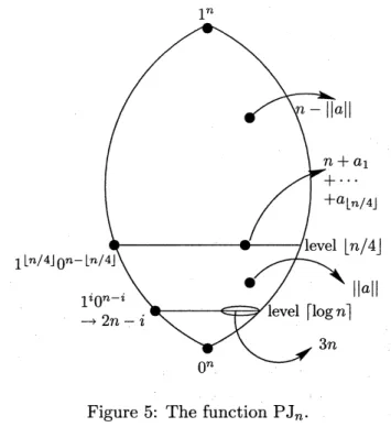
probability. The function is called$\mathrm{P}\mathrm{J}_{n}$ (path and

jump) and is defined in the following way (see

Figure 5). Definition 7 $PJ_{n}(a)=\{$ $3n$ $if||a||=k$ and $a_{1}+\cdots+a_{k}=0$ $2n-i$ _if$a=1^{i}0^{n-i}$_,

$0\leq i<\lfloor n/4\rfloor$ $n+a_{1}+\cdots+a_{\mathrm{L}^{n}/4\rfloor}$ $if||a||=\lfloor n/4\rfloor$ $||a||$ $if||a||<\lfloor n/4\rfloor$ and

$a$ does not belong

to theprevious cases

$n-||a||$ otherwise.

where $k=$ rlog$n1$.

Theorem 9 The optimal static mutation

prob-ability equals $(\ln n)/(4\cdot(\ln 2)\cdot n)$ leading to an

expectedrun time

_of

the $(1+1)EA$ $of\ominus(n^{2361}\cdots)$.

The expected run time

_of

the dynamic $(1+1)EA$ $equals\ominus(n^{2}\log n)$.

The search procedure works as follows. It is

rather easy to find the level $\lfloor n/4\rfloor$, a mutation

probability of $1/n$ is good for this purpose. On

cepted while sitting in a trap are the other trap

points and $1^{n}$. Finally, ajump of length at least

$n/8$flippingexactly all zerosis necessarytoreach

$1^{n}$. All not mentioned points _$a$ have a fitness of $n-||a||$.

It is unlikely that the dynamic $(1 +1)\mathrm{E}\mathrm{A}$

reaches the trap before reaching the path.

How-ever, while passing the path it is very likely to

reach the trap which leads to an exponentialrun

time with very high probability. The (I+I)EA

with mutation probability $1/n$ also reaches the

path with high probability before reaching the

trap. Sitting on the path it is very unlikely to

reach the trap whose distance is at least $n/16$.

Hence, with overwhelming probability the global

optimum is reached in polynomial time.

Figure 5: Thefunction $\mathrm{P}\mathrm{J}_{n}$.

We haveto exchange zeros from the first quarter

with ones from the rest. Again mutation prob-abilities of approximately $1/n$ are good for this

purpose and the same holds for the short path

with increasingfitness valuesfrom $1\lfloor n/4\rfloor \mathrm{o}n-\mathrm{L}^{n}/4\rfloor$

to $0^{n}$. Finally, we have to flip rlog_$n1$ zeros (not

from the first rlog$n1$ positions) simultaneously.

Then a mutation probability of $\ominus((\log n)/n)$ is

appropriate. The dynamic $(1 +1)\mathrm{E}\mathrm{A}$ has

dur-ing each phase for each situationone stepwith a

good mutation probability. A good static

muta-tion probabilityhas to be acompromise between

a good choice for the early stages and a good

choice for the last jump.

However, the dynamic (I+I)EA can be a dis-aster for functionswhich canbe solved efficiently

with a static $(1 +1)\mathrm{E}\mathrm{A}$ with mutation

proba-bility $1/n$. The corresponding function is called

$\mathrm{P}\mathrm{T}_{n}$ (path with trap). Again, we consider the

path from $0^{n}$ to 1n containing all points $1^{i}0^{n-\acute{l}}$.

Except some holes with fitness $0$ the fitness of

the points equals $n+\dot{i}$ and 1n is the global

op-timum with fitness $3n$. The holes are chosen

to guarantee that the algorithm cannot pass the

path too quickly. The trap consists of all points

which can be reached from some point

1i

$0^{n-i}$,

$n/4\leq\dot{i}\leq 3n/4$, if approximately $n/8$ bits flip

simultaneously and which have a Hamming

dis-tance of at least $n/16$ to the path. The trap

points have a fitness of $2n$. The only points

ac-9

Crossover

really

can

help

,

Jansen and Wegener (1999) were the first to

provethat uniformcrossovercan decrease therun

timeofevolutionaryalgorithmswithoutcrossover from superpolynomial to polynomial.

Definition 8

_Uniform

crossover applied to

$x,$$x’$ $\in$ $\{0,1\}^{n}$ produces the random point

$x”$ $\in$ $\{0,1\}^{n}$ where the bits $x_{i}’’$ are chosen

independently and $x_{i}^{\prime;}=x_{i}$,

if

$x_{i}=x_{i}’$, and $Pr(x_{i}^{J}’=0)=Pr(x_{i}^{J}’=1)=1/2$ otherwise.

Definition 9 The

_function

$JUMP_{m,n}$ is

defined

$by$

$JUMP_{m,n}(a)=\{$

$||a||$ $\dot{i}f||a||\leq n-m$ or $||a||=n$

$n-||a||$ otherwise.

We only consider the case where $m=o(n)$.

Then it is very likelythat the initial population

ofpolynomial size only contains individualswith at most $n-m$ ones. Individuals with more than $n-m$ ones and less than $n$ ones will not be

ac-cepted. Hence, the global optimum has to be

produced from individuals with at most $n-m$

ones. Mutations have difficulties with this task.

The expected time for the nlutation probability

$1/n$ is bounded below by $n^{m}$ and a lower bound

of $\Omega(n^{m-\in}),$ $\epsilon>0$, for the general case can be

obtained easily.

What about uniform crossover? If we have two

no common zero, uniform crossover produces 1n

with probability $2^{-2m}$ and the probability that

a mutation step with mutation probability $1/n$

doesnot destroy1n is approximately $e^{-1}$. Hence,

uniformcrossoverworkswell, moreprecisely leads

to expectedpolynomialtimeiftheindividuals are

randomlstrings with $m$ zeros and $m=O(\log n)$.

The difficulty is the so-called hitchhiking effect.

Because of selection andcrossover theindividuals

are not independent and have a larger chance of

(

$‘ \mathrm{o}\mathrm{v}\mathrm{e}\mathrm{r}\mathrm{l}\mathrm{a}\mathrm{p}\mathrm{p}\mathrm{i}\mathrm{n}\mathrm{g}$zeros”.

Therefore, Jansen and Wegener (1999)have

in-vestigated a genetic algorithmwith thevery small

crossover probability$p_{C}=1/(.n\log n)$. The

algo-rithm works as follows.

Algorithm 2 Steady state genetic algorithm

with crossover probability $p_{c}=1/(n\log n)$ and

mutation probability $p_{m}=1/n$. The population

size is $n$ and the population is initialized

ran-domly. The main loop

_of

the algorithm looks as

follows:

2.

_If

$m$ $=$ $O(\log n)$, the expected run time

is bounded by $O(n\log n(3n\log n2+2^{2m}))=$

$poly(n)$.

For tlueproofof thisbound we describea

“typ-ical run” of the genetic $\mathrm{a}_{\mathrm{o}\mathrm{r}\mathrm{i}}\mathrm{t}\mathrm{h}\mathrm{n}1$starting with

an arbitrary initial population. A typical run

should reach the optimum within a given time

bound. We describe the events leading to a

non-typical run and estimate the corresponding “fail-ure probability”. Ifthe sum of failure

probabili-tiesis bounded above by $1-\delta,$ $\delta>0$, the success

probabilityfor the considered number ofsteps is at least $\delta$. If the search

was.

not successful, we

start the next phase. Since theinitial population

wasassumedto be arbitrary, we can usethesame

estimates. Hence, the expected numberofphases

canbe estimated above by$\delta^{-1}$. In ourcase, _$1-\delta$

is even $o(1)$.

For $\mathrm{J}\mathrm{u}\mathrm{m}_{\mathrm{P}m,n}$, a typical run consists of three

phases where the length ofall phases is bounded

$\dot{\mathrm{a}}\mathrm{b}\mathrm{o}\mathrm{v}\mathrm{e}$

by the stated asymptotic bounds. A

typical run has $\mathrm{t}\dot{\mathrm{h}}\mathrm{e}\mathrm{f}\mathrm{o}\mathrm{i}1_{\mathrm{o}\mathrm{W}\mathrm{i}}\mathrm{n}\dot{\mathrm{g}}$ properties:

- after phase 1, we either have found the

op-timum or the population only contains indi-viduals with exactly$n-m$ones (this implies

for all further phases that we only accept

in-dividuals with $n-m$ ones or the optimum),

- after phase 2, we either have found the

op-timum orthe population only contains

indi-vidualswith exactly$n-m$onesandfor each

bit position there are at most $n/(4m)$

indi-viduals with a zeroat this position (the zeros

are sufficiently well spread),

The choice

_of

the parents or the parent can be

done randomly or

_fitness

based. The selection

procedure is the following one.

_If

$\dot{t}he$ new

indi-vidual $x$ equals one

of

its parents, it is rejected.

Otherwise, it replaces one $of.the$ worst individuals

$y$

if

$f(x)\geq f(y)$.

Theorem 10 The steady state genetic algorithm

has

_for

$JUMP_{m,n}$ the following behavior.

1.

_If

$m$ $=$ $O(1)$, the expected run time is

bounded by$O(n^{2}\log n)$.

- during phase 3, we either find the optimum

or the population only contains individuals

with exactly$n-m$ ones andfor eachbit

po-sition there are at most $n/(2m)$ _individuals

witha zero at this positionandat the endof

phase 3 the optimumis found.

Theanalysisofphase1iseasyusing thecoupon

collector’s theorem. If the condition ofphase3 is

fulfilled, the probability that two randomly

cho-senparents (or fitness based chosen parents which

is the same, since the fitness of all individuals

1/2 and uniform crossover can work. The

anal-ysis of phase 2 is the difficult task (the difficult

part of the analysis ofphase 3 can be performed

similarly). We consider only bit position 1, all

other positions lead to the same failure

probabil-ities. Hence, the total failure probability can be

boundedby$n$times thefailureprobabilityfor bit

position 1.

We denote by $p^{-}(z)$ and $p^{+}(z)$ the

probabil-ity that the number of individuals with a zero at

bit position 1 decreases by 1 resp. increases by 1

duringone step starting with$z$individualswitha

zero at bit position 1. Inorder to estimate these probabilities we have to perform quite exact cal-culations. Since $p_{c}$ is small enough, we can

con-sider acrossover stepas a “badevent” increasing

the number of zeros at position 1. The result of

the calculations is that

$z\geq n/(8m)\Rightarrow$ $p^{-}(z)=( \frac{1}{n})$ and

$p^{-}( \mathcal{Z})-p^{+}(z)=\ominus(\frac{1}{n})$ .

Hence, either $z<n/(8m)$ and we are far away

from a failure or $z\geq n/(8m)$ and we havealarge

enoughtendencytodecreasethe number of zeros.

The precisecalculations leadtothe desired result.

Conclusions

We have argued why the analysisofevolutionary

algorithms should be performed just as the

anal-ysis of other randomized algorithms and search

heuristics. Several examplesof new results, some of them proving or disproving well-known

con-jectures, others leading to results ofa new type,

prove that this approach is worth to be followed

further.

References

[1] B\"ack, T. (1993). Optimal mutation rates in

genetic search. Proc. of 5th ICGA (Int. Conf.

on Genetic Algorithms), 2-8.

[2] B\"ack, T. (1998). An overview of parameter

control methods by self-adaptation in

evolu-tionary algorithms. Fundamenta Informaticae

35, 51-66.

[3] B\"ack, T., Fogel, D. B., and Michalewicz, Z.

(Eds). (1997). Handbook

_of

Evolutionary

Com-putation. Oxford Univ. Press.

[4] Beyer, H.-G. (1996). Toward a theory of

evo-lution strategies: Self-adaptation. Evoevo-lution-

Evolution-ary Computation 3, 311-347.

[5] Droste, S., Jansen, T., and Wegener, I. (1998a). A rigorous complexity analysis of the $(1+1)$ evolutionary algorithm for

separa-ble functions with Boolean inputs.

Evolution-ary Computation 6, 185-196.

[6] Droste, S., Jansen, T., and Wegener, I.

(1998b).On the optimization of unimodal

func-tions with the $(1+1)$ evolutionary algorithm.

Proc. of PPSN V (Parallel Problem Solving from Nature), LNCS 1498, 13-22.

[7] Fogel, D. B. (1995). Evolutionary Computa-tion: Toward a NewPhilosophy

_of

Machine In-telligence. IEEE Press.

[8] Goldberg,D. E. (1989). Genetic Algorithmsin

Search, Optimization, and

_Mac.hine

Learning. Addison Wesley.

[9] Holland, J. H. (1975). Adaptation in

Natu-ral and

_Artificial

Systems. The University of

Mic.higan

Press.

[10] Horn, J., Goldberg, D. E., and Deb, K. (1994). Long path problems.Proc. of PPSNIII (Parallel

Proble.m

Solvingfrom

_Nature.)

$-$

, LNCS

866, 149-158.

[11] Jansen, T., and Wegener, I. (1999). On the analysis of evolutionary algorithms –a proof

that crossover really can help. Proc. of ESA

’99 (European Symp. on Algorithms), LNCS

1643, 184-193.

[12] Jansen, T., and Wegener, I. (2000a). On

the choice of the mutation probability for the

$(1+1)\mathrm{E}\mathrm{A}$. Proc. of PPSN VI (ParallelProblem

Solving from Nature), LNCS 1917, 89-98. [13] Jansen, T., and Wegener, I. (200ob).

Evolu-tionaryalgorithms-howtocopewith plateaus

of constant fitness and when to reject strings

ofthe same fitness. Submitted to IEEE Rans.

on Evolutionary Computation.

[14] Mitchell, M., Forrest, S., and Holland, J. H. (1992). The Royal Road function for genetic

algorithms: Fitness landscapes and GA

per-formance. Proc. of 1st European Conf. on

[15] Mitchell, M., Holland, J. H., and Forrest, S.

(1994). When will a genetic algorithm

outper-form hill climbing. In: Cowan, J., Tesauro, G.,

and Alspector, J. (Eds): Advances in

Neu-ral Information Processing Systems. Morgan

Kaufmann.

[16] Motwani, R., and Raghavan, P. (1995).

Ran-domized$Alg_{\mathit{0}}r\dot{i}ihms$

.

Cambridge Univ. Press.

[17] M\"uhlenbein, H. (1992). How genetic

algo-rithms really work. I. Mutation and $\mathrm{h}\mathrm{i}\mathrm{l}\mathrm{l}\mathrm{c}\mathrm{l}\mathrm{i}\mathrm{m}\mathrm{b}\vee-$

ing. Proc. of PPSN II (Parallel Problem

Solv-ingfrom Nature), 15-25.

[18] Rabani, Y., Rabinovich, Y., and Sinclair, A.

(1995).A computational view of population ge-netics. Random Structures and Algorithms 12, 314-334.

[19] Rosenberg, I. G. (1975). Reduction of

bi-valent maximization to the quadratic case.

Cahiers du Centre d’Etudes de Recherche

Op-erationelle 17, 71-74.

[20] Rudolph, G. (1997). How mutations and

se-lection solvelong path problemsin polynomial

expected time. Evolutionary Computation 4,

195-205.

[21] Schwefel, H.-P. (1995). Evolution and

Opti-mum Seeking. Wiley.

[22] Wegener, I., and Witt, C. (2000). On the

behavior of the $(1+1)$ evolutionary algorithm

on

quadratic pseudo-boolean functions.

Sub-mitted to Evolutionary Computation.

[23] Wolpert, D. H.,andMacready,W.G. (1997).

No free lunch theorems for optimization. IEEE