Exploration and application of GRACE terrestrial water storage product for hydrologic studies in regional scale 利用統計を見る

(1)

EXPLORATION AND APPLICATION OF GRACE

TERRESTRIAL WATER STORAGE PRODUCT FOR

HYDROLOGIC STUDIES IN REGIONAL SCALE

(地域スケール水文解析に対する GRACE 陸域貯水量情報の

適用方法の検討)

山梨大学大学院

医学工学総合教育部

博士課程学位論文

2015 年 9 月

NING SHAOWEI

(2)

EXPLORATION AND APPLICATION OF GRACE

TERRESTRIAL WATER STORAGE PRODUCT FOR

HYDROLOGIC STUDIES IN REGIONAL SCALE

地域スケール水文解析に対する

_GRACE

陸域貯水量情報の適用方法の検討

A dissertation submitted in partial fulfillment of the requirements for the degree of Doctor of Philosophy in Engineering

Special Doctoral Course on Integrated River Basin Management Interdisciplinary Graduate School of Medicine and Engineering

University Of Yamanashi, Japan

September 2015 NING SHAOWEI

(3)

(4)

i

ABSTRACT

Recently, terrestrial water storages from Gravity Recover And Climate Experiment (GRACE) remote sensing satellite has become available for water resource monitoring. The GRACE mission, jointly operated by NASA and the German Aerospace Center, launched on March 17, 2002 and has continued to perform past its nominal mission lifetime of five years GRACE has the ability to quantify changes of terrestrial water storage, which is the sum of groundwater, soil moisture, surface water, snow, ice, and vegetation biomass, representing a new source of information for hydrologists and the global hydrological modeling community. To date, there are many researches focusing on using GRACE data on global and continental scale for different kind of hydrologic studies such as estimating evapotranspiration based on terrestrial water budget equation over large river basin and constraining global scale land surface model. But, they are not enough.

The main objective of this thesis is to explore some potential applications of GRACE based terrestrial water storage product in a number of hydrological and environmental studies over a number of regional scale East Asia catchments. We first introduced the theory behind GRACE satellite, operating mechanism of GRACE mission, GRACE data and provided detailed TWS retrieval procedure from GRACE GSM data. Then three case studies relevant to GRACE data application in regional scale were discussed:

1. Downscaling of GRACE terrestrial water storage using satellite and GLDAS products

The application of GRACE data for local-scale water resources management has been limited because of its coarse resolution. The purpose of this case study is to investigate the feasibility of downscaling GRACE with a statistical method.

(5)

ii

Study area chosen followed two criteria. Firstly, study area should locate in the range of 30°N~30°S, where P is a dominant control on terrestrial water storage change and GRACE derived water storage change had good correlation with P, ET and R according to previous researches. Secondly, it should encompass continuously monitored wells as many as possible in the extent of gridded GRACE pixel (1°×1°), because groundwater level change can reflect local water storage change well then it can be a good indicator to validate downscaling performance. So a 1-degree GRACE pixel at 102-103︒E and 24-25︒N within which located five monitoring wells was chosen as the downscaling study area, water storage change (ΔS) derived by water balance equation was calculated from TRMM 3B43 products, MODIS Global Evapotranspiration Project (MOD16) ET product and runoff output of GLDAS-Noah land surface hydrological model. Then empirical regression methods based on the relationship between GRACE and other hydrological fluxes were applied to downscale a 1 degree gridded GRACE product to 0.25°. Observed groundwater level data were used to validate the downscaling performance. Results indicated that GRACE TWS had good relationship with storage change obtained by water balance equation. Statistical regression downscaling method for GRACE can provide more fine spatial information of water storage change effectively.

2. Calibration a hydrologic model by step-wise method using GRACE TWS and discharge data

The objective of this case study is to propose a new calibration procedure for a basin-scale hydrological model using GRACE derived terrestrial water storage data and observed discharge data.

Study area of this case study is the Da River Basin (DRB) located in subtropical regions which is the biggest tributary of the Red River with the basin area of 55,000 km2 and originates from mountainous region in Yunnan Province, China. The model used here was developed based on the Hydrological Predictions for the Environment (HYPE) model. We modified the HYPE model to calculate total water storage by adding up all water components that can be simulated such as snow, soil moisture, groundwater, water in channels and lakes. The analysis was conducted in a step-wise calibration method within Differential Evolution Monte Carlo Markov Chain simulation framework. Two groups of parameters (3 for each group) sensitive to

(6)

iii

water storage simulation and runoff generation respectively were calibrated in three steps: First, calibrated model derived TWS with GRACE derived one in monthly scale over 2003 to 2006 to get optimal value of three parameters with close relation to water storage. Second, fixed parameters obtained from the first step and calibrated for two stations’ discharge to optimize another three parameters pertinent to runoff generation. Third, combined the six parameters to get the final calibration result. Finally, by comparison with conventional calibration method, this calibration approach efficiently reduce parameter uncertainty, model can perform good discharge simulation and reasonable water storage simulation. We also found that based on this method, our model can enhance actual and potential evapotranspiration simulation in sub-basin scale. More important, this case study demonstrated the potential for the joint use of available GRACE derived water storage data and discharge data to improve main hydrological flux simulations in hydrologic models.

3. Remote sensing based analysis of recent variations in water resource and vegetation of a semi-arid region

In this case study, we focused on the analysis of a combination of free available satellite data including GRACE TWS, TRMM, MODIS/Landset, satellite altimetry data (T/P, Jason-1/2) and NDVI coupled with in situ climate data to assess the water resource variation within a sparsely gauged area -- Hulun lake region and its impact on eco-environment then provide useful information for future water resource management and eco-environmental protection. The results showed that GRACE TWS data was adequate to capture the water resource variation in this region and was consistent with precipitation change pattern. Based on the general understanding about water resource variations, we checked the response of Hulun lake. Results indicated that lake level and lake surface area both declined quickly during 2002 to 2009, with about 3 meter of water level declination and 400km2 of lake surface shrinkage respectively and then trended to be stable after 2009 even through precipitation had recovered back to pre-2002 level. We can infer that water resource condition needed more time and precipitation recharge to recover from a drought attack in this typical semi-arid region. Furthermore, the vegetation response to water resource variations reflected that resilience and drought resistance ability of the vegetation in most regions were high. Drought hazard did not bring seriously negative implications on vegetation growing condition. Only 16.5% of the study area

(7)

iv

where locates north and west of Hulun lake and northwest mountain areas showed vegetation degradation.

In this thesis, we introduced how to calculate terrestrial water storage from the original GRACE spherical harmonic coefficients and explored three pertinent applications of the GRACE remote sensing satellite for hydrological studies over a number of East Asia regions of regional scale. From these three case studies, 1) A framework of statistical regression downscaling of GRACE TWS data using freely available satellite and land surface model products was developed and explored in a low altitude area. The results showed that this method could provide more fine spatial information of water storage change effectively. 2) A new calibration procedure for a basin-scale hydrological model using GRACE derived terrestrial water storage data and observed discharge data was proposed. 3) A framework for estimating water resource variation in spatial–temporal and its impact on eco-environment using only freely available remote sensing data (including GRACE) in less gauged semi-arid area was provided and this methodology can be adapted in other regions.

Key words: GRACE, terrestrial water storage, statistical downscaling, hydrological model calibration, water resource variation analysis

(8)

v

ACKNOWLEDGEMENT

Looking back on the fantastic journey of past three years, I found I could not gone so far without continuous help and strong support from many people. It is a great pleasure for me to thank for their scientific guidance, encouragement and patience.

First of all, I would like to express my topmost thankful to my supervisor, Associate Professor Hiroshi Ishidaira. His guidance, support, and inspiration from the very beginning to the concluding stage of this dissertation enable me to develop an understanding of the research topic. During my Ph.D. studies, his intelligent, optimistic and diligent research attitude deeply influenced me. He is more than an academic supervisor for me, but also a life mentor. Especially, I learned from him how to accomplishment the research through individual thinking, which would benefit me for the rest of my life.

I further express my gratitude to all the Professors and researchers in International Research Center for River Basin Environment (ICRE), University of Yamanashi, who instructed, helped and encouraged me in various ways during my doctoral study. My heartfelt appreciation goes to all members of my senior seminar: Professor Y. Sakamoto, Professor T. Suetsugi, Professor J. Shindo, Associate Professor Y. Ichikawa, Associate Professor K. Nishida, Dr. J. Magome, Associate Prefessor. K. Souma, Dr. I. Inagaki, Dr. T. Sano, Dr. T. Nakamura, and Dr. V. Pandey. I also would like to specially thank the retired Professor K. Sunada for his helpful guidance and encouragement.

I would like to express my gratitude to all my friends in ICRE group, who accompany, support and encourage me during my life in Japan. My sincere thanks go to Dr. J. Wang, Dr. T. Khujanazarov, Dr. R.A. Kristanti, Dr. M. Sujata, Dr. D.T. Nga, Dr. D.N. Khoi, Dr. Kakizawa, Dr. Y. Wijayanti, Mr. S. Manandhar, Dr. L. Li, Dr. S. Salina, Dr. R. Setyawaty, Dr. S. Park, Dr. M. Hashimoto, Dr. Y. Li, Dr. S. Heng, Dr. H. Widyasamratri, Dr. S. Shrestha, Dr. D. Amarathunga, Mr. Udmale, Ms. T.H. Bui, , Ms. N.T.P. Mai, Mr. Nguyen Minh Vuong, Ms. Nguyen Y Nhu, Mr. Tatsuru Kamei, Mr. Ebata Kazunori, Mr. Shankar Shrestha, Mr. Bhesh Raj Thapa, Mr. Luis Alfaro,

(9)

vi

Ms. Hein,Ms. Rawintra Eamrat , Mr. Bikesh Malla, Ms. Nurul Nadiah Binti Norzon, Mr. Yuya Takabe, Mr. Tomoaki Kozono and Mr. Takehiro Okamoto.

I would like to give my sincere gratitude to Associate Professor G.Q. Wang, Professor H.Q. Wang and Professor Z.X. Xu, who recommended me to study in Japan, and keeps encouraging and supporting me during my Ph.D. study. As well, I want to acknowledge my wife and my parents, their love and support enabled me to overcome the frustrations of last three years.

Last but not least, thanks to ICRE group and Ministry of Education, Culture, Sports, Science and Technology (MEXT) and for the financial support during the study period.

(10)

vii

LIST OF FIGURES

Figure 1.1 Potential ways in which remote sensed observations can inform water resource assessment systems ... 4 Figure 1.2 GRACE: water equivalent thickness (cm) for July, 2011 over land (Jin S. et al., 2013) ... 5 Figure 2.1 Time series of TWS anomalies (mm) from GRACE for Amazon (Falvio et al. 2012) ... 12 Figure 2.2 Trends in GRACE TWS over period August 2002 to December 2011 (Jin et al., 2013) ... 12 Figure 3.1 An overview of mass transport, mass variations, and exchange in the earth system (Panet et al., 2012) ... 20 Figure 3.2 Different satellite tracking missions. High–low satellite-to-satellite tracking in the CHAMP mission (Left). Low-low satellite-to-satellite-to-satellite-to-satellite tracking in the GRACE mission (Right) (From http://www.csr.utexas.edu/grace/) .. 21 Figure 3.3 Internal view of GRACE satellite instruments (From http://www.csr.utexas.edu/grace/)... 22 Figure 3.4 GRACE mission data flow (CSR/TSGC Team Web, 2012) ... 23

Figure 3.5 Data sample of GRACE level – 2 provided by JPL ( File name: GSM-2_2003001-2003031_0026_EIGEN_G---_0005) ... 25 Figure 3.6 (1) Spatial pattern of mass variation in October 2013 from GRACE GSM SH coefficients, no destriping and Gaussian smoothing applied. (2) Same as (1), but a 400 km Gaussian smoothing applied. (3-6) Same as (2), but destriping methods from Swenson and Wahr (2006), Chambers and Bonin (2012), Chen et al. (2007a) and Duan et al. (2009) applied. ... 32 Figure 3.7 Flow chart to calculate TWS derived from the GRACE data ... 35

(14)

xi

Figure 3.9 Study area for comparison between GRACE derived TWS and land

surface model derived TWS ... 36

Figure 3.10 Schematic figure of Noah land surface model (http://www.nar.ucar.edu/2012/lar/ral/) ... 37

Figure 3.11 Time series of TWS from GRACE and Noah model ... 37

Figure 3.12 Relation between GRACE TWS and Noah derived TWS ... 37

Figure 4.1 Location of the study area... 43

Figure 4.2 Statistical downscaling framework ... 45

Figure 4.3 The monthly GRACE TWS and ∆S series of study area over period of 2007 to 2012 ... 48

Figure 4.4 The regression equation of monthly ∆S and GRACE TWS at 1 degree scale. ... 48

Figure 4.5 16 GRACE TWS anomaly series of downscaled grids at 0.25°scale with line color corresponding to location color. ... 49

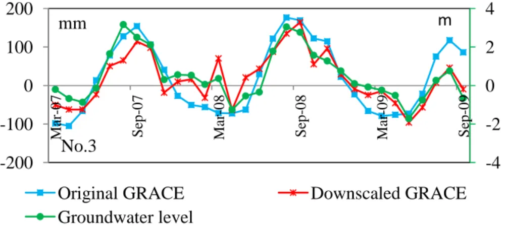
Figure 4.6 Comparison of measured groundwater level deviations（right axis）with downscaled and original GRACE TWS anomalies (left axis). ... 50

Figure 4.7 Downscaled total water storage change for study area in March 2008. .. 52

Figure 5.1 Location of the study area and the meteorological stations ... 59

Figure 5.2 Schematic figure of basin water movement procedure in HYPE model and model structure within one HRU (Lindstrom et al., 2010). ... 61

Figure 5.3 Schematic figure of step-wised calibration method used in this chapter 62 Figure 5.4 Flow chart of Differential Evolution Markov Chain Monte Carlo algorithm ... 63

Figure 5.5 Probability density function of parameters in the first step of the calibration (a) and second step (b) ... 64

Figure 5.6 GRACE TWS and model derived TWS for the whole DRB in step-wise calibration ... 65

(15)

xii

Figure 5.8 Probability density function of parameters in the traditional calibration using discharge only ... 67 Figure 5.9 GRACE TWS and model derived TWS for the whole DRB in traditional calibration ... 68 Figure 5.10 Observed potential ET and model derived under two calibration methods (a) traditional, (b) step-wise ... 69 Figure 5.11 Actual ET (derived by AA method) and model derived under two calibration methods (a) traditional, (b) step-wise ... 70 Figure 6.1 The geographic location and STRM-based elevation map of the study area (red color region in the down figure shows the Eurasian steppe zone). ... 78 Figure 6.2 Vegetation map of study area ... 78

Figure 6.3 EOF decomposition of TWS changes over the study area. EOF patterns show in left side and corresponding unit-less temporal patterns (PCs) in right side. 88 Figure 6.4 EOF decomposition of precipitation changes derived from TRMM satellite data over study area EOF patterns show in left side and corresponding unit-less temporal patterns (PCs) in right side... 90 Figure 6.5 Annual precipitation and water storage changes series from 2002 to 2012 ... 91 Figure 6.6 Temperature trend analysis for whole study area ... 91

Figure 6.7 (a) Lake water level, (b) lake water surface area and (c) correlation between lake water level and surface area ... 93 Figure 6.8 Spatial distribution of average NDVI (a) and trends of inter-annual NDVI change over 2002 to 2012 (b) ... 95

(16)

xiii

LIST OF TABLES

Table 3.1 Level-2 GSM data information, red color means data missing, yellow color indicates low quality, green color means data normal. ... 34 Table 4.1 R2 between groundwater level deviation series and original GRACE TWS anomaly series, downscaled GRACE TWS anomaly series respectively ... 50 Table 5.1 HYPE hydrologic calibration parameters ... 62

Table 5.2 Performance of two different calibration approaches for discharge simulation ... 67 Table 5.3 R2 between observed series and model derived series for two different calibration methods respectively ... 70 Table 6.1 Observed precipitation stations and their correlation with TRMM precipitation ... 89 Table 6.2 Comparison of MODIS and LANDSAT derived Hulun lake area ... 92

(17)

xiv

LIST OF ABBREVIATIONS

GRACE Gravity Recover And Climate Experiment TRMM Tropical Rainfall Measurement Mission

MODIS Moderate resolution Imaging Spectro-radiometer AVHRR Advanced Very High Resolution Radiometer GLADS Global Land Data Assimilation System EOF Empirical Orthogonal Function

HYPE Hydrological Predictions for the Environment SLR Satellite Laser Range

NDVI Normalized Difference Vegetation Index MNDWI Modified Normalized Difference Water Index DEMCMC Differential Evolution Markov Chain Monte Carlo

(18)

1

(19)

(20)

3

1.1 Background

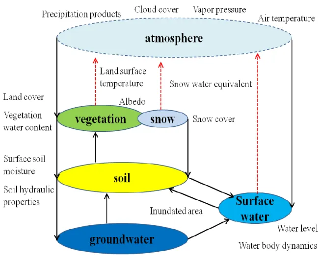
Land surface hydrology is an accounting of the water received (precipitation) and water lost (evaporation, runoff from land, streams to oceans) and the gain in water storage (rise in level of inland water bodies, increase in soil moisture, snow and, rise in water table). This accounting is based on a simple water balance principle, i.e. a conservation of mass. Understanding each hydrological variable and its processes for estimating and predicting water resource variations based on water balance method in a river catchment has become one of the major tasks for hydrologists since the 18th century. However, one of big obstacles here is that quantification of each hydrological flux exactly over large spatial domains and over long time periods is extremely difficult due to measurement complications. Such as, point observed precipitation is inadequate to stand for regional spatial distributed precipitation. In addition, each of the components that we measured has a degree of uncertainty. This error in the various components can further spread into a significant uncertainty in the total water storage estimate and hydrologic modeling. Luckily, this problem has been partially addressed with the evolution of satellite observation technique (Kumar et al., 2013).

With the successful launch of the first Earth Resources Technology Satellite (ERTS-1 or Landsat-1) on 23 July 1972, scientists and engineers gained a valuable new source of space-based observations for studying hydrologic systems and processes. Satellite remote sensing provides lots of spatial data products like land use type, evaporation, surface temperature, snow water equivalent, water storage change, vegetation index and so on. Those products often allow for the advantage of observing hydrologic variables in a distributed way, offering a different view with respect to traditional observations that can help with understanding and modeling the hydrological cycle. Moreover, remote-sensing data are fundamental in scarce data environment (Fernandez et al., 2012). Remote sensing application also helps to improve the hydrological modeling by providing vital information about precipitation, soil moisture content and ET rates (as Figure.1.1 shows), meanwhile conversely, calibrating and assimilating hydrological or land surface model with these remote sensing derived variables also become a very hot research topic (Dijk et al. 2011).

(21)

4

Figure 1.1 Potential ways in which remote sensed observations can inform water resource assessment systems

Recently, a new global remote sensing dataset has become available for water resource monitoring and hydrological model calibration. This dataset is the derived terrestrial water storages from Gravity Recover And Climate Experiment (GRACE) remote sensing satellite. The GRACE mission, jointly operated by NASA and the German Aerospace Center, launched on March 17, 2002 and has continued to perform past its nominal mission lifetime of five years. GRACE was designed as a geodesy mission to measure the gravitational field of the earth at first. As we know, the main drivers of temporal variations in the gravity file are oceanic and atmospheric circulations and redistribution of terrestrial water via hydrological cycle. So by accounting for the first two using analysis models, GRACE has the ability to quantify changes of terrestrial water storage, which is the sum of groundwater, soil moisture, surface water, snow, ice, and vegetation biomass (shown in figure 1.2),

(22)

5

representing a new source of information for hydrologists and the global hydrological modeling community (Jin S., 2013).

Figure 1.2 GRACE: water equivalent thickness (cm) for July, 2011 over land (Jin S., 2013)

1.2 Necessity of the study

As no global complete network of surface hydrological observations exists, the advances of satellite gravimetry to monitor terrestrial water storage are significant and unique for determining changes in total water storage and water balance closure at global and continental scales. To date, there are many researches focusing on using GRACE data on global and continental scale for different kind of hydrologic studies such as estimating evapotranspiration based on terrestrial water budget equation over large river basin and constraining global scale land surface model. But, they are not enough. To explore the potential applications of GRACE based terrestrial water storage product in a number of environmental and hydrological studies at regional scale is very necessary.

(23)

6

This thesis will pioneer some of the most pertinent applications of the GRACE remote sensing satellite for hydrological studies over a number of East Asia catchments of varying spatially scales. Hence, the specific objectives of the study are as follows:

(1) To calculate terrestrial water storage from the original GRACE spherical harmonic coefficients and use land surface model derived soil moisture content to validate our result in tow main of our study area.

(2) To test if it is possible to downscale 1 degree resolution GRACE TWS grid product into finer resolution, therefore get more detailed TWS information in spatial scale.

(3) To design a new hydrological model calibration method with GRACE TWS as one calibration target to improve hydrological model performance and reduce model parameter uncertainty.

(4) To combine the available GRACE TWS, in situ climate data, MODIS, TRMM, satellite altimetry data (T/P/Jason-1/2), and high resolution Regional Climate simulations data to assess the water storage changes within Hulun lake region and its impact on ecological environment then provide useful information for future water resource management and environment protection.

1.4 Organization of the dissertation

To accomplish the above-mentioned objectives, this thesis is structured in seven chapters. The brief content and outline of these chapters is presented as follows:

Chapter 1: Introduction

This chapter introduces the application of remote sensing technique in hydrological study, emphasizes GRACE satellite’s contribution to hydrological research. In addition, motivation and necessary of the study, objectives of the research, structure of the thesis are also presented. In this chapter, the organization of dissertation is proved to give the overview of the study.

(24)

7

This chapter summarizes the main relevant information and previous research about various applications of GRACE data in hydrological research. They are delineated in 5 topics, including: Application in continental hydrology and validation; Estimation of goe-hydrological parameters; Estimates of snow mass changes at high latitudes; Optimization and assimilation into hydrological models.

Chapter 3: GRACE mission and TWS data calculation

In this chapter, an introduction about theory behind GRACE and GRACE data is presented. In addition, the full process of TWS calculation is described in detail. Validation of TWS calculated above with water storage derived from land surface model (Noah) is conducted at last.

Chapter 4: Downscaling of GRACE Terrestrial Water Storage Using Satellite and GLDAS Products

In this chapter, we investigated the feasibility of downscaling GRACE with a statistical method. Empirical regression methods based on the relationship between GRACE and other hydrological fluxes were applied to downscale a 1 degree gridded GRACE product to 0.25°. Observed groundwater level data were used to validate the downscaling performance. Results indicated that GRACE TWS had good relationship with storage change obtained by water balance equation. Statistical regression downscaling method can improve GRACE data resolution effectively.

Chapter 5: Calibration of a Hydrologic Model by Step-wise Method Using GRACE TWS and Discharge Data

In this chapter, we proposed a new calibration procedure for a basin-scale hydrological model using satellite-derived terrestrial water storage data and observed discharge data. The analysis was conducted in a step-wise calibration method within Differential Evolution Monte Carlo Markov Chain simulation framework. In comparison with conventional calibration method, this approach efficiently reduce parameter uncertainty, model can perform good discharge simulation and reasonable water storage simulation. In addition, based on this method, the model can enhance actual and potential evapotranspiration simulation in sub-basin scale.

(25)

8

Chapter 6: Remote sensing based analysis of recent variations in water resource and vegetation of a semi-arid region

In this chapter, we focus on the analysis of a combination of free available satellite data including GRACE TWS, TRMM, MODIS/Landset, satellite altimetry data (T/P, Jason-1/2) and NDVI coupled with in situ climate data to assess the water resource variation within a sparsely gauged area -- Hulun lake region and its impact on eco-environment then provide useful information for future water resource management and eco-environmental protection.

Chapter 7: Summary of the study

This chapter summarizes the results and contributions of the study, and then gives suggestions for the future study.

(26)

9

(27)

(28)

11

2.1 Introduction

Terrestrial water storage is a major component of global hydrological cycle which plays an important role in the Earth’s climate system by controlling over water, energy and biogeochemical fluxes. However, even then, TWS is not well-know at regional and global scales in consequence of the lack of in situ observations and systematic monitoring of the terrestrial water component, especially the groundwater part (Alsdorf and Lettenmaier, 2003). Although some local hydrological monitoring networks exist, the current insight into water storage comes basically from global hydrological models (e.g. WaterGAP Global Hydrological Model) or Global Land Data Assimilation Sytem - GLDAS, which still suffer from various limitations, for example, the absence of different compartments of the terrestrial water compartments (e.g., groundwater and floodplains), the errors introduced by input forcing data like precipitation, the parameterization. Now that GRACE has already offered a unique alternative to classical remote sensing technique for measuring changes in TWS, it is worthy of taking full advantage of TWS data to test and explore its application in diverse hydrological and relevant studies. In the following sections of this chapter, a review of GRACE’s major application in hydrological studies is proposed.

2.2 Application in continental hydrology and validation

Once sufficiently long series of GRACE solutions were made available, various studies for validating these products were made. In general, GRACE-based estimates of TWS compare favourably with those based on land surface models as well as atmospheric and terrestrial water balances (Rodell et al., 2004; Ramillien et al., 2005; Syed et al., 2005; Klees et al., 2008). Besides model calculated water storage, surface water level and groundwater table changes all are suitable water storage change indicator that can be used for comparison with GRACE TWS. Correlations of up to 0.8 between GRACE-based TWS and measurements of more than 230 station gauged water level along the Amazon River were found by Flavio et al.(2012). Combined with other satellite techniques such as imagery, GRACE geoid data were used to study the mechanisms of seasonal flooding in large inundation areas like the Mekong delta (Frappart et al., 2006) and large river basins as the Amazon River, Fig

(29)

12

2.1 (Frappart et al., 2008; Papa et al., 2008). In addition, by analyzing the spatial and temporal trend of TWS, GRACE also has been used widely to monitor water resource depletion. Research shows that north part of India and China, west coast of USA have all been suffering severe water stocks shrinking in recent decade, Fig 2.2 (Jin, 2013).

Figure 2.1 Time series of TWS anomalies (mm) from GRACE for Amazon (Falvio, 2012)

Figure 2.2 Trends in GRACE TWS over period August 2002 to December 2011 (Jin, 2013)

(30)

13

2.3 Optimization and assimilation into hydrological models

The GRACE data have been widely confronted to global hydrological outputs for comparison and validation, and then to improve the description and parameterization of the hydrological processes in the models. The GRACE data were used as a proxy to test and improve the efficiency of surface waters schemes in the ORCHIDEE land surface hydrological model (Ngo-Duc et al., 2007).

Guntner(2008) pointed out the importance of integrating the GRACE data into hydrological models for improving the reliability of their prediction through advanced methods of objective calibration and data assimilation. A multi-calibration approach to constrain model predictions by both measured river discharge and TWS anomalies from GRACE was applied to the WGHM model, improving simulation results with regard to both objectives. Using only monthly TWS variations, the RMSE was reduced of about 25mm for the Amazon, 6mm for the Mississippi and 1mm for the Congo river basins (Werth et al., 2009). Lo et al. (2010) incorporated both GRACE TWS and estimated base flow data in the calibration of Community Land Model (CLM 3.0), demonstrated the advantages gained from this approach using a Monto Carlo simulation framework. His approach improved parameter estimation and reduced the uncertainty of water table simulations in the CLM. Besides these studies focused on calibrating global land surface model using GRACE TWS, some researchers found that incorporating TWS as one calibration objective in distributed hydrological model (like SWAT) calibration for mesoscale river basin could also improve model performance in some extent (Xie et al., 2012, Lei et al., 2013, Milzow et al., 2011).

GRACE derived monthly TWS anomalies were also assimilated into one of the GLDAS models using Kalman smoother method by Zaitchik in 2008. Compared with open loop simulations, assimilated ones provided better performance thanks to improvements in the surface and groundwater estimates (Zaitchik et al., 2008). (Forman et al., 2012) assimilated GRACE TWS into Catchment Land Surface Model over the Mackenzie River basin located in northwest Canada. Assimilation was conducted with an ensemble Kalman smoother (EnKS).Model estimates with and without assimilation are compared against independent observational data sets of snow water equivalent and runoff. For snow water equivalent, modest improvements

(31)

14

in mean difference and root mean square error were achieved as a result of the assimilation.

2.4 Estimation of goe-hydrological parameters

GRACE based estimates of river discharges are based on the solution of the water balance equation at basin scale:

2.1

Where, S is terrestrial water storage (TWS), P and ET the basin wide totals of precipitation and evapotranspiration, and R the total basin discharge, or the net surface and groundwater outflow.

As ET presents large uncertainties, the quantity P-ET is eliminated using the water balance of the atmospheric branch of the water cycle:

2.2

Where, W is the vertically integrated precipitable water, the divergence of the vertically integrated average atmospheric moisture flux vector, computed using the following equations:

2.3

2.4

Where, and are the pressure at the surface and top of the atmosphere respectively, q is the specific humidity, g is gravitational acceleration and the horizontal wind vector.

This approach was firstly applied to the Amazon and the Mississippi river basin (Syed et as., 2005), and extend to obtain a global volume of freshwater discharge estimated here is 30,354 ± 1,212 km3/y (Syed et as., 2009).

GRACE based TWS can be also used to estimate changes in vertical water fluxes solving the water balance equation (Equ.2.1). Changes of regional evapotranspiration (ET) rate over Mississippi basin were estimated by combining GRACE TWS data

(32)

15

with observed precipitation and steamflow in the water balance equation (Rodell et al., 2004). Similarly, (Ramillien et al., 2005) solved the water balance equation for ET rate. Time variations of ET were evaluated over 16 drainage basins solving the water balance equation and using precipitation from GPCC and runoff from the WGHM model (Doll et al., 2003), and they revealed that GRACE based ET variations were comparable to the ET value simulated by four different global hydrological models. Swenson and Wahr (2006) estimated the difference precipitation minus evapotranspiration using the water balance framework and comparing to surface parameters variations from global analysis.

2.5 Estimates of glacier snow changes at high latitudes

After distinguishing water and snow contributions from observed gravity field by use of an inverse iterative approach based on the least-squares criteria, Frappart et al. (2006) used satellite microwave data and global hydrological model outputs to validate GRACE-derived glacier snow mass changes at high-latitudes. In particular, RMS errors of 10-20mm were found for Yenisey, Ob, Mckenzie and Yukon basins. Comparison at basin scales between GRACE-derived glacier snow mass variations, GRACE-based TWS variations and river discharge temporal evolution shows that the glacier snow component has very obvious influence on river discharge at high latitudes than TWS, and that glacier snow and river discharge show similar inter-annual variability (Frappart et al., 2011).

2.6 Contribution of TWS to sea level variations

Seasonal and inter-annual changes in land water storage derived from GRACE were used to estimate the contribution of land hydrology to the sea level variations for 27 of the largest drainage basins in the world. Estimation of 2002-2006 sea level contribution of GRACE TWS of Amazon basin was made, and corresponded to a water loss of ~ 0.5mm per year (Ramillien et al., 2008). Wouters et al.(2011) recently estimated the global mean eustatic cycle, i.e., the total amount of water exchanged between continents and ocean, to be 9.4 ±0.6 mm equivalent water level over the period 2003-2010.

(33)

16

This chapter here briefly introduces the applications of GRACE satellite data in various hydrological related studies. Altogether, these studies clearly demonstrate that gravity estimates from GRACE, can be used to improve hydrological studies in global or large continent scales. It is worth noting that very few studies focus on exploring any potential applications of GRACE satellite output in regional hydrological and environmental studies.

(34)

17

CHAPTER 3 GRACE Mission and TWS

Data Calculation

(35)

(36)

19

In this chapter, we introduce the reader about theory behind GRACE satellite, operating mechanism of GRACE mission and GRACE data. In addition, the full process of TWS calculation is described in detail. Comparison between TWS calculated above and water storage derived from land surface model (Noah) is conducted at last.

3.1 Background

In physics, gravitation or gravity is the tendency of massive objects to accelerate toward each other. Earth’s gravitational attraction keeps the moon and satellites in orbit around the Earth. The gravitational force exerted between two objects can be determined using Newton’s law of gravity as below equation:

Where, G is the magnitude of the gravitational force between the two objects, K is the universal gravitational constant (6.6726 × 10-11 Nm2kg-2), m1 is the mass of object 1 in kg, m2 is the mass of a second object 2 in kg and r is the distance between the two object in m. The force of gravity is weak compared with the other forces in nature, such as electric and magnetic forces, but gravity’s influence is the most far reaching and dramatic. Sea level variations (SLV), melting of polar ice caps and mountain glaciers, extreme droughts and floods - these and those issues of global climate change are closely related to the gravity variations on the Earth. Detailed knowledge on gravity variations caused by mass transport and redistribution among continents, oceans, atmosphere and cryosphere will help us better understand the physics of global climate change (Figure 3.1). Therefore, the precise measurement of gravity is very important for geodetic applications and a number of important aspects for global change.

3.2 The Gravity Recovery and Climate Experiment (GRACE)

3.2.1 Mission objective and follow-on

The twin GRACE satellites were launched in March 2002 as a joint US/NASA-German/DLR (Deutsches Zentrum für Luft- und Raumfahrt) project. The design

(37)

20

lifetime was 5 years, and the mission objectives were to accurately map the global gravity field every 30 days (Tapley et al., 2004a). Furthermore, a minimum science requirement was to deliver a new model of the Earth’s static geoid with an error of less than 1 cm, within the first year (Davis et al., 1999).

Figure 3.1 An overview of mass transport, mass variations, and exchange in the earth system (Panet et al., 2012)

Well beyond the first 5 years of operation, the GRACE mission has recently been extended to the year 2013. The outstanding performance that GRACE has shown to monitor mass movements on and near the Earth’s surface, has led the US National Research Council Decadal Survey to recommend a GRACE-Follow-On mission for launch around 2017–2020 (Cazenave and Chen, 2010). Meanwhile, a GRACE-Gap-Filler mission is considered for launch around 2015 (Cazenave and Chen, 2010; Tapley et al., 2010).

3.2.2 Satellite-to-satellite tracking (SST)

The Earth’s gravity field has for a long time been studied through satellite orbit perturbations, observed with GPS satellites and ground-to-satellite lasers. When one satellite in a low Earth orbit (LEO), is being tracked by satellites in higher orbits (like the GPS satellites), the mission is called a high-low satellite-to-satellite tracking

(38)

21

mission (HL-SST). GRACE however, is a so-called low-low satellite-to-satellite tracking (LL-SST) mission, where two identical LEO satellites co-orbit, with an inter-satellite distance of a few hundred kilometers. LL-SST is a relatively new development in the estimation of gravity fields, and GRACE is in fact the first mission of its kind. Figure 3.2 shows the difference of these two tracking missions. For gravity recovery, Spherical Harmonic (SH) methods usually include GPS data, making the gravity solution a combined LL and HL product. For the Mascon method, GPS data is not used.

Figure 3.2 Different satellite tracking missions. High–low satellite-to-satellite tracking in the CHAMP mission (Left). Low-low satellite-to-satellite-to-satellite-to-satellite tracking in the GRACE mission (Right) (From http://www.csr.utexas.edu/grace/)

In general, SST methods rely on the relationship between the parameters of the terrestrial gravity field (typically Clm and Slm coefficients will be introduced in next section) and the observables from the satellite tracking (Seeber, 2003), which in the case of the GRACE mission is the relative velocity of the two satellites.

Because the GRACE satellites travel in the exact same orbit, only displaced by a few hundred kilometers, relatively local anomalies can be observed compared to SST missions where only one LEO satellite is used. When the GRACE satellites pass over a mass anomaly on or near the surface of the Earth, the leading satellite senses the anomaly first as it causes a small perturbation in the orbit. Shortly after, the trailing satellite experiences the exact same perturbation caused by the same anomaly, only slightly displaced in time. Hence, the residual created by the anomaly in the GRACE

(39)

22

K-Band Range-Rate (KBRR) data (the change in inter satellite distance) is centered exactly on top the anomaly (Lemoine et al., 2007; Rowlands et al., 2010).

The orbital height has a great effect on the resolution of the gravity field that can be recovered from the tracking data. The lower the orbit, the better the resolution, but also the more drag on the satellites and the shorter life time. The GRACE satellites were launched at an initial hight of approximately 500 km as a compromise of reduced drag and reduced resolution of gravity anomalies.

3.2.3 Instrumentation

Figure 3.3 Internal view of GRACE satellite instruments (From

http://www.csr.utexas.edu/grace/)

The key element of the GRACE mission is measurement of the inter-satellite distance, as variations in the distance are caused by non-uniformities in the Earth’s gravitational field. To accurately measure the distance, a K-Band Ranging System is placed on each satellite, facing towards the other satellite. It transmits a signal of known frequency and wavelength to determine the inter-satellite distance. The transmitted signal is then reflected on the other satellite, and the difference in phase

(40)

23

between the transmitted and the reflected signal is measured, in order to determine the distance.

Orbit perturbations are not only caused by the Earth’s gravitational pull, but also by more direct factors like atmospheric drag and thrusting events. These factors are a source of error in estimating the gravity field from measurements of the inter-satellite distance. To measure the non-gravitational accelerations of the spacecrafts, an accelerometer is placed on both satellites. Additional ancillary instruments include GPS receivers for precise time-tagging and positioning, and attitude sensors which provide high precision inertial orientation of the satellites (Tapley et al., 2004a).

3.3 GRACE data

(41)

24

The initial data processing of the GRACE science data, is being handled by the three processing centers within the GRACE Science Data System (SDS): the NASA Jet Propulsion Laboratory (JPL), the Center for Space Research at the University of Texas, Austin (UTCSR), and the Geoforschungszentrum in Potsdam, Germany (GFZ). The SDS is designed to perform all tasks for gravity field processing to the production of monthly and mean gravity fields (Bettadpur et al., 2007b). The data products are being categorized according to the processing level that has been applied. Figure 3.4 shows the procedure of GRACE data collection, process, integration and issuance.

3.3.1 Level-0 data

The level-0 data is the raw GRACE data product, continuously passed to the GRACE Raw Data Center (RDC) at DLR in Neustrelitz. This data is divided into a scientific instrument stream and a spacecraft housekeeping stream, and placed in a rolling archive. From here, the SDS centers transfer the data to their own permanent archives (Bettadpur, 2007a). The interesting data for gravity field estimations are the inter satellite range-rate measurements (mm/s), but also accelerometer data and attitude and positioning data are important.

3.3.2 Level – 1A data products

The level-1A processing step includes time-tagging to the satellite receiver clock and time-tag ambiguity corrections are performed. Furthermore the data is reformatted, and quality and editing control flags are added. This processing step is nondestructive, and the processing can be reversed to obtain the original level-0 data if desired, except for bad data packets. Ancillary data products needed for further processing are also included in the level-1A data (Bettadpur, 2007b).

3.3.3 Level – 1B data products

The level-1B data is correctly time tagged and the sample rate is reduced. As for the level-1A data, level-1B data includes ancillary data needed for further processing. The level-1B processing is possibly irreversible (Bettadpur, 2007b). For the mascon method, which will be described in detail in chapters 6 and 7, the level-1B data is used to fit Mascon parameters through a least squares inversion.

(42)

25

3.3.4 Level – 2 data products

The level-2 data product includes all gravity field and related products, derived from the previous processing level products. Ancillary data is also included (Bettadpur, 2007a). A GRACE Level-2 gravity field product is a set of spherical harmonic (SH) coefficients of the exterior geopotential. A product name is specified as:

PID-2_YYYYDOY_YYYYDOY_dddd_ssss_mmmm_rrrr

Where, PID is a 3 characters product identification mnemonic. – 2 denotes a GRACE Level – 2 product. YYYYDOY_YYYYDOY specifies the date range (in year and day – of – year format) of the data used in creating this product. dddd is the (leading-zero-padded) number of calendar days from which data was used in creating the product. ssss is an institution specific string. mmmm is a 4-character free string (e.g. used for distinguishing constrained from unconstrained solutions). rrrr is a 4 – digit (leading –zero –padded) release number (0000, 0001, …)

Figure 3.5 Data sample of GRACE level – 2 provided by JPL ( File name: GSM-2_2003001-2003031_0026_EIGEN_G---_0005)

The Product Identifier mnemonic (PID) is made up of one the following values for each of its 3 characters:

(43)

26

1st Character: G—Geoptential coefficients.

2nd Character: S—Estimate made from only GRACE data, C – Combination estimate from GRACE and terrestrial gravity information, E – Any background model specified as time series, A – Average of any background model over a time period.

3rd Character: M—Estimate of the static field, U—Geopotential estimate relative to the background gravity model, T—Total background gravity model except for background static model, A—non-tidal atmosphere, B—non-tidal oceans, C— Combination of non-tidal atmosphere and ocean, D—bottom-pressure over oceans, zero over land.

Till now, there are totally 6 categories of level 2 data can be download online. Their PIDs are GAA, GAB, GCM, GAD, GSM, GAC. These data are all in format of GRCOF2. Figure 3.5 shows one example data of GSM been used for TWS calculation in this study. The first line gives the name of this data file, it including PID, the starting time and ending time that this data was created. The second shows the product type. The third line gives the information about deviations. The fourth line provides two parameters about the Earth, the first one is reference earth mass and the second is average diameter of the Earth. The fifth line gives some simple information about the data, they are fully normalized spherical harmonic coefficients of static gravity model till to 90 order and degree. From the sixth line to the end of file it lists the data that can be used for TWS calculation, the first two number columns are degree and order then next two columns are spherical harmonics coefficients ( ,

3.4 Temporal Gravity Field and TWS calculation

3.4.1 Basic of temporal gravity field

The gravitational potential of the earth has been modeled with the Laplace equation in spherical coordinates, which is given blow:

(44)

27

Where, N is the gravitational potential, r is the distance from the origin of the coordinate system, θ is the latitude, and is the longitude. The gravitational potential of the earth is commonly described in terms of the shape of the geoid. A geoid, often referred to as a close representation or physical model of the earth’s shape, is an equipotential surface which approximately coincides with the mean ocean surface. The geoid can be expressed as a sum of spherical harmonics:

Where, , are Earth’s radius, co-latitude and longitude, respectively; l, m are

degree and order; , are spherical harmonic (SH) coefficients (i.e., Stokes coefficient); and are fully normalized associated Legendre functions.

The temporal variation of geoid ( can also be described as changes of SH

coefficients ( ):

We define as the variation of mass density in a thin layer of the Earth’s

surface:

Which is the radial integral of density redistribution -- . Then we expand as a sum of coefficients:

(45)

28

Where is the density of water (1000 kg m-3). The ratio of is defined as the equivalent water thickness (EWT), which is often used for GRACE applications.

Suppose the observable mass redistribution of the Earth occurs within the thin surface layer, the SH coefficients of geoid change is a combination of direct gravitational attraction of surface mass change and an additional contribution caused by the solid Earth’s loading effect (Chao et al., 1987; Farrell, 1972):

Where is the load Love number of degree , is the average density of the Earth (5517 kg m-3 ).

Comparing equation 3.6 and 3.7, it is easy to find the relation between

( ) and ( ):

Or, conversely,

Finally, we can find the change of surface mass density from changes of the geoid SH coefficients ( ):

(46)

29

Equation 3.10 can be used to estimate the change of surface mass density (or in EWT, we assume that the main mass redistribution is induced by water storage change, so calculated EWT can also stand for the terrestrial water storage change ) from geoid SH coefficients provide by GRACE gravity field solutions (Such as GSM product mentioned in previous section). By the way, usually the EWT or TWS is calculated as 1 degree resolution grid data. We also should note that all temporal gravity signals originate from the Earth’s surface. Since most mass fluctuations of the Earth occurs in atmosphere, cryosphere, ocean and upper crust within a 10 to 15 km layer, thin layer assumption is reasonable.

3.4.2 Post-processing Methods 3.4.2.1 Gaussian Smoothing

Gaussian filter on the sphere was firstly developed by Jekeli (1981) to smooth the Earth’s gravity field. Then, lots of researchers adopted Jekeli’s Gaussian smoothing method to process Stokes coefficients of GRACE temporal gravity files. In this method, the spatial average of the surface mass density is expressed as follows:

Where, is an averaging function. Combing equation 3.10 and 3.11,

it gives Where,

(47)

30

If is defined as a function of angle between points ( ( ,

equation 3.12 can be simplified as:

3.14 Where,

Where, = / are the Legendre polynomials.

We adopt Jekeli’s Gaussian average function but normalized it so that global integral of W is 1, so we get:

Where, is the Earth’s radius, is the Gaussian average radius which is the

distance on the Earth’s surface at which decreases to half of its value at = 0. The recursion relations among are:

(48)

31

3.4.2.2 Destriping Methods

In spatial domain, original unconstrained monthly gravity field observed by GRACE shows north-south stripes, which represent the correlated errors in the gravity coefficients. As an example, spatial pattern of mass variations in October 2013 from original GRACE SH coefficients is shown in Figure. 3.6. Swenson and Wahr (2006) found that, for a given order m, SH coefficients of the same parity are correlated with each other. They proposed a method to reduce this correlation by using quadratic polynomial in a moving window of width w centered at degree l, For example, for , they used the Stokes coefficients ,…, , , , …, to fit a quadratic polynomial, and removed the fitted value from original to derive the de-correlated . The relation between the width of moving window w (the number of coefficients used for quadratic polynomial fitting) and α is w = 2α + 1. In the paper of (Swenson and Wahr, 2006), the detailed algorithm to determine the width of moving window was not provided. Referring to Swenson and Wahr’s unpublished results, (Duan et al., 2009) provided the window width in the form showing below:

Where, m is order (≥5), takes the larger one of the two arguments. Swenson and Wahr have empirically chose A = 30 and K = 10 based on a trial and error procedure.

To estimate ocean mass change using GRACE, (Chambers et al., 2006) modified the algorithm described above. For RL02 GRACE GSM product, they keep 7×7 portion of the coefficients unchanged, and fit a 7th order polynomial to the remaining coefficients to degrees with the same parity for each order up to 50. In their method, only one polynomial is used for each odd or even set for a given order, unlike the method from (Swenson and Wahr et al., 2006). For RL04 GRACE GSM product, they keep 11×11 portion of the coefficients unchanged, and a 5th order polynomial is applied. For latest RL05 GRACE solutions, the optimal parameterization based on the model test is to start filtering at degree 15, and adopt a 4th polynomial (Chambers and Bonin, 2012). This processing method is denoted as P4M15.

(49)

32

(Chen et al., 2007a) used the P3M6 method to process GRACE data and estimated coseismic and post-seismic deformation from the Sumatra-Andaman earthquake using GRACE. Later, they adopted the P4M6 method to estimate mass balance in ice caps, mountain glaciers, and terrestrial water storage change (Chen et al., 2009a, 2010a, 2007b, 2008, 2009b, 2010b).

Figure 3.6 (1) Spatial pattern of mass variation in October 2013 from GRACE GSM SH coefficients, no destriping and Gaussian smoothing applied. (2) Same as (1), but

a 400 km Gaussian smoothing applied. (3-6) Same as (2), but destriping methods from Swenson and Wahr (2006), Chambers and Bonin (2012), Chen et al. (2007a)

and Duan et al. (2009) applied.

Different from the above methods, (Duan et al., 2009) determined the unchanged portion of coefficients based on the error pattern of the coefficients. Their unchanged portion of coefficients and the width of moving window depend on both degree and order in a more complex way. As a example, Figure 3.6 shows the global mass variations in October 2013 from GRACE Stokes coefficients based on different

(50)

de-33

striping methods. As shown in Figure 3.6(3-6), there is a general agreement among results from different de-striping methods. In addition, de-striping process suppresses the north-south stripes more efficiently, comparing the results with only the Gaussian smoothing applied.

In summary, the parameterization of de-striping (or de-correlation) method for GRACE is dependent on the following criterion: (a) Determination of unchanged portion of coefficients: (Swenson and Wahr, 2006, Chambers and Bonin, 2012 and Chen et al., 2007a) keep the first 4, 14 and 5 degree and order unchanged respectively; while (Duan et al., 2009) determined the unchanged portion of coefficients based on their error pattern, which depends on both degree and order. (b) Choice of the degree of polynomial fitting; (c) How to apply the polynomial fitting to coefficients (moving window vs. fixed window): (Swenson and Wahr, 2006) adopted a moving window with the width, which depends on the degree; while (Duan et al., 2009) determined the width of moving window as a function of both degree and order. In addition, (Chambers, 2006 and Chen et al., 2007a) did not move the window, but used a fixed window to fit the polynomial.

In addition, many filters are designed to constrain the noise of GRACE solutions, e.g., classic Gaussian filter (Jekeli, 1981), non-isotropic filter (Han et al., 2005), statistical filter (Davis et al., 2008), DDK filter (Kusche, 2007), wavelet filter (Schmidt et al., 2006), wiener filter (Sasgen et al., 2007), fan filter (Zhang et al., 2009), and so on. In this thesis, we mainly adopt (Duan et al., 2009)’s de-striping method and fan filter to estimate regional terrestrial water storage variations inferred from GRACE level 2 - GSM product.

3.4.3 TWS calculation

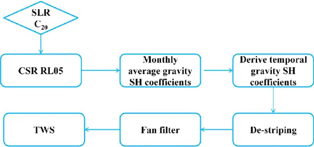
Based on the previous section, the calculation of TWS from GRACE data will be presented in this section. In our study we used the Level-2 monthly GSM product from Center for Space Research at the University of Texas (UTCSR) to retrieve TWS. The data information was shown in Table 3.1. Data period is from 2003 to 2012, but there are several month that data are missed, they are May-2003, January, June-2011, May, October-2012. In addition, because of satellite orbit coverage problem in January 2004, data quality in this month is very bad. To get the high accurate TWS results, we eliminate data of this month.

(51)

34

Table 3.1 Level-2 GSM data information, red color means data missing, yellow color indicates low quality, green color means data normal.

CSR RL05 1 2 3 4 5 6 7 8 9 10 11 12 2003 2004 2005 2006 2007 2008 2009 2010 2011 2012

After download the GSM SH coefficients, we can start to calculate TWS. Figure 3.7 shows the main steps of calculation procedure.

First, substitute the C20 term of GSM data, because the C20 term of GRACE data is not highly accurate. (Chen et al., 2008) indicated that from the comparison between C20 from GRACE and SLR, C20 from SLR showed significant seasonal variability. So for the sake of high calculation accuracy, we chose C20 from SLR to substitute original C20 from GRACE.

Second, get monthly average gravity SH coefficient. We decided the average gravity field of 2003 – 2009 as reference gravity field. Monthly average gravity SH coefficient was calculated by averaging the SH coefficients of 72 month over 2003 to 2009.

Third, get the temporal gravity SH coefficients. The TWS was derived from these temporal gravity SH coefficients, they were calculated by subtracting average gravity SH coefficient from original gravity SH coefficients over period 2003 to 2012.

Finally, after get the temporal gravity SH coefficients they were processed by de-striping and Fan filter then substituted into equation 3.10 to get the TWS in 1 degree resolution.(As Figure 3.8 shown).

(52)

35

Figure 3.7 Flow chart to calculate TWS derived from the GRACE data

Figure 3.8 Global water storage change map derived from GRACE

3.4.4 TWS Validation

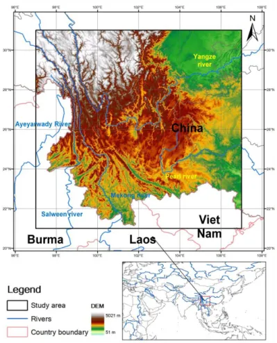
To validate our GRACE derived TWS, we compared it with land surface model derived TWS in the area as Figure 3.9 shown below, which covers two of our study area in the next two chapters.

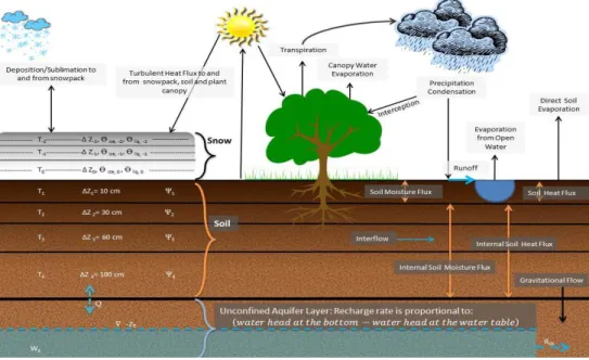
The land surface model used here is Noah model, it is used widely in simulating the dynamics of soil moisture, plant physiology, micrometeorolgy, and the interactions between atmosphere, biosphere and hydrosphere. Figure 3.10 shows the

(53)

36

schematic of Noah model, for detail information, reader can refer to paper of (Chen et al., 1996). It should be noted that Noah model derived TWS here only includes soil moisture, canopy water storage and snow water equivalent, it is not really same as GRACE derived TWS. But these three water component account for main part of TWS on land and its variation can significantly reflect TWS. So it is reasonable to compare GRACE derived TWS with Noah model derived TWS to check the performance of TWS we calculated from GRACE. The Noah model water storage components can be downloaded from Global Land Data Assimilation System (GLDAS).

Figure 3.9 Study area for comparison between GRACE derived TWS and land surface model derived TWS

The results shown in Figure 3.11 and 3.12 indicated that GRACE derived TWS matched with model derived TWS very well over period from 2003 to 2012. The R square value between the two data series was up to 0.80. This also guaranteed that our GRACE derived TWS was adequate for detecting and monitoring water storage.