Atomic-resolution imaging in liquid by frequency modulation atomic force microscopy using small cantilevers with megahertz-order resonance frequencies

frequency modulation atomic force microscopy using small cantilevers with megahertz‑order resonance frequencies

著者 Fukuma Takeshi, Onishi K., Kobayashi N., Matsuki A., Asakawa Hitoshi

journal or

publication title

Nanotechnology

volume 23

number 13

page range 135706

year 2012‑04‑06

URL http://hdl.handle.net/2297/31369

doi: 10.1088/0957-4484/23/13/135706

Atomic-resolution imaging in liquid by frequency modulation atomic force microscopy using small cantilevers with megahertz-order resonance

frequencies

T Fukuma

, K Onishi

, N Kobayashi

, A Matsuki

and H Asakawa

1Frontier Science Organization, Kanazawa University, Kakuma-machi, Kanazawa 920-1192, Japan

2Division of Electrical and Computer Engineering, Kanazawa University, Kakuma-machi, Kanazawa 920-1192, Japan

3Bio-AFM Frontier Research Center, Kanazawa University, Kakuma-machi, Kanazawa 920-1192, Japan

E-mail: [email protected]

Abstract. In this study, we have investigated the performance of liquid-environment FM-AFM with various cantilevers having different dimensions from theoretical and experimental aspects. The results show that the reduction of the cantilever dimensions provides improvement in the minimum detectable force as long as the tip height is sufficiently long compared with the width of the cantilever. However, we also found two important issues to be overcome to achieve this theoretically-expected performance.

The stable photothermal excitation of a small cantilever requires much higher pointing stability of an excitation laser beam than that for a long cantilever. We present a way to satisfy this stringent requirement using a temperature controlled laser diode module and a polarization-maintaining optical fiber. Another issue is associated with the tip.

While a small carbon tip formed by electron beam deposition (EBD) is desirable for small cantilevers, we found that an EBD tip is not suitable for atomic-scale applications due to the weak tip-sample interaction. Here we present that the tip-sample interaction can be greatly enhanced by coating the tip with Si. With these improvements, we demonstrate atomic-resolution imaging of mica in liquid using a small cantilever with a megahertz-order resonance frequency. In addition, we experimentally demonstrate the improvement in the minimum detectable force obtained by the small cantilever in the measurements of oscillatory hydration forces.

PACS numbers: 07.79.Lh, 68.37.Ps

1. Introduction

Frequency modulation atomic force microscopy (FM-AFM)[1] has traditionally been used for atomic-scale investigations on various materials in vacuum[2]. However, recent advancements in its instrumentation[3] have made it possible to operate FM-AFM with true atomic resolution even in liquid[4], which has opened up new applications in chemistry[5, 6] and biology[7, 8, 9, 10, 11, 12, 13, 14, 15]. To obtain true atomic- resolution images by FM-AFM, it is required to detect short-range interaction force acting between the tip front atom and surface atom. Althogh the minimum detectable force (F

) required for it depends on various conditions, it typically falls in the range of 10–100 pN. In vacuum, this condition can be easily satisfied due to the high Q factor of the cantilever resonance (Q = 1,000–100,000). However, this can barely be satisfied in liquid even with the optimal operating conditions owing to the low Q factor (Q = 1–10). Such a narrow margin of the performance often leads to the low efficiency and reproducibility in experiments and practically limits the application range.

The theoretical limit of F

in FM-AFM is ultimately determined by the cantilever parameters such as Q, resonance frequency (f

) and spring constant (k)[1]. Among them, k is often determined by the application purpose so that it is often impossible to vary it for the improvement in F

. The enhancement of Q-factor in liquid generally leads to an increase of k, giving little improvement in F

. Thus, previous efforts have mainly been focused on the enhancement of f

to obtain a higher force sensitivity and faster time response. One of the major strategies for this is to reduce the cantilever size.

By reducing the cantilever size in an appropriate manner, f

can be increased without giving a significant change in k and Q.

Although advantages of using a small cantilever have theoretically been expected, it was practically very challenging at the early stage of AFM development. However, now the situation has been changed by the technical advancements. Several groups have presented practical ways to fabricate small cantilevers with a high resonance frequency[16, 17, 18]. In addition, several sophisticated designs for low noise and wideband deflection sensors for small cantilevers have been proposed[19, 20, 3, 21, 22, 23].

So far, applications of small cantilevers have mainly been focused on the high- speed imaging in liquid using amplitude modulation AFM (AM-AFM)[24, 16, 25].

These previous works demonstrated the improved time response of dynamic-mode AFM obtained by the small cantilevers. However, the advantages of using small cantilevers also include the improvements in F

. Thus, it should also be effective for improving F

in FM-AFM. To date, there have been no reports on the atomic-scale FM-AFM applications using small cantilevers with megahertz-order f

in liquid. Therefore, it has remained unclear if there are any practical issues that may prevent such an application.

For example, it has not been experimentally verified if the enhancement of f

actually provides the theoretically expected improvement. Due to the hydrodynamic

damping caused by the water squeezed between a cantilever and sample surface,

significant reduction of Q is expected[26, 27, 28], which may cancel out the improvement obtained by the enhanced f

. Such “squeeze film effect” may become prominent when a small cantilever with a short tip is used.

Another important issue is the stability. The atomic-scale applications typically require higher stability than the high-speed applications. Thus, it has been questioned if such a high stability can be obtained with a small cantilever with a high f

. In particular, in FM-AFM, a cantilever is driven with a feedback circuit based on the phase of the cantilever deflection signal. Therefore, the stable operation of FM-AFM imposes more stringent requirements on the detection and excitation of the cantilever oscillation than in the case of AM-AFM.

Furthermore, some of the recently developed small cantilevers have a carbon tip formed by electron beam deposition (EBD). All of the atomic-scale FM-AFM images reported so far have been obtained by a Si tip. Thus, it has been unclear if such an EBD tip is applicable to atomic-scale applications.

In this study, we aim at improving F

obtained in liquid by FM-AFM using small cantilevers having a megahertz-order f

. First, we compared the FM-AFM performance obtained by various cantilevers having different dimensions near and far from the sample surface. We discuss the improvement obtained by the reduction of the cantilever size from both theoretical and experimental aspects. Secondly, we clarify the practical issues to be overcome for applying a small cantilever to atomic-scale FM-AFM experiments:

instability of the cantilever excitation and weak interaction between an EBD tip and surface. We also present ways to overcome these difficulties. Finally, we demonstrate stable atomic-resolution FM-AFM imaging of a cleaved mica surface in liquid using a small cantilever. In addition, we experimentally demonstrate the improvement in F

obtained by the small cantilever in the measurements of oscillatory hydration forces.

2. Experimental details

The scanning electron microscopy (SEM) images of the cantilevers were obtained by S-

3000N (Hitachi). The AFM experiments were performed by a custom-built AFM head

with an ultralow noise cantilever deflection sensor[3, 29] and a photothermal excitation

setup[30]. The AFM head was controlled with a commercially available AFM controller

(ARC2: Asylum Research). This controller was also used for the measurements of

frequency spectral density distributions. The cantilever excitation was performed with

a commercially available oscillation controller (OC4: SPECS). This controller was also

used for the measurements of deflection spectral density distributions. The FM-AFM

imaging was performed with a constant frequency shift (∆f) mode. During the imaging

the cantilever oscillation amplitude (A) was kept constant. The sample used for the

FM-AFM imaging was a round disk of muscovite mica (01877-MB: SPI Supplies).

3. Improvement obtained by small cantilevers 3.1. Calculations from cantilever dimensions

(d) USC

100 µm (a) NCH

(c) UHF

(b) NCVH 20 µm

20 µm 20 µm

20 µm

100 µm 100 µm

100 µm

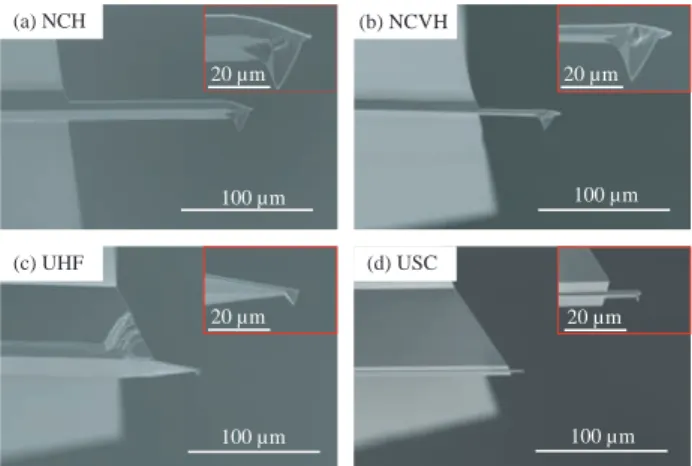
Figure 1. SEM images of the cantilevers used in this study.

Table 1. Cantilever dimensions measured from SEM images. The UHF cantilever has a triangular shape so that the averaged width is given in the table. k,f₀^∗ andQ^∗ were calculated from the cantilever dimensions and equations (1), (3) and (4). F_min^∗ was calculated from these parameters and equation (10). B = 100 Hz. T = 298 K.ρ = 997.044 kg/m³. µ= 0.89 mPa·s. E= 170 GPa (NCH, NCVH and UHF) or 76.3 GPa (USC).ρc = 2330 kg/m³(NCH, NCVH and UHF) or 3700 kg/m³ (USC).

` w t h H k f₀^∗ Q^∗ F_min^∗

[µm] [µm] [µm] [µm] [N/m] [MHz] [pN]

NCH 136.4 30.2 3.69 13.9 0.46 25.6 0.13 6.0 4.2 NCVH 60.5 13.2 1.86 13.0 0.98 17.4 0.34 4.7 2.4

UHF 34.4 20.7 1.27 4.2 0.20 — — — —

USC 11.1 4.8 0.82 2.2 0.46 29.0 2.83 5.0 1.0

In this experiment, we used four different types of cantilevers supplied by Nanoworld (Neuchˆ atel, Switzerland): NCH, NCVH, UHF and USC (prototype). Figure 1 shows SEM images of the cantilevers. The cantilever dimensions (length: `, width:

w, thickness: t, tip height: h) were measured by other SEM images with higher magnifications (not shown here) as shown in table 1. Among the four cantilever types, NCH is the largest and most commonly used for atomic-scale FM-AFM imaging in liquid as well as in vacuum[31]. USC is the smallest one and has recently been developed for high-speed AFM applications. UHF has a triangular shape while the others have a rectangular shape. The width of the UHF cantilever described in table 1 is the average value, namely, a half of the width measured at the fixed end of the cantilever.

From the cantilever dimensions, k, f

and Q can be calculated with several

assumptions. Assuming that the cantilever has a uniform rectangular cross section

and no tip, k and f

in vacuum are given by[2]

k = Ewt

4`

, (1)

f

= 0.162 t

`

s

E ρ

, (2)

where E and ρ

denote the Young’s modulus and density of the cantilever material.

The resonance frequency and Q-factor in liquid (f

and Q

) are generally much smaller than the values in vacuum and given by[32]

f

= f

q

1 + (πρw/4ρ

t)Γ

, (3)

Q

= (4ρ

t/πρw) + Γ

Γ

, (4)

where ρ denotes the density of the liquid. Γ

and Γ

are the real and imaginary parts of the hydrodynamic function and given by[32, 27]

Γ

= 1.0553 + 3.7997

√

Re , (5)

Γ

= 3.8018

√

Re + 2.7364

Re . (6)

(7) Re denotes the modified Reynolds number and given by[32]

Re = πρf

w

2µ , (8)

(9) where µ is the viscosity of the liquid.

From these equations and the cantilever geometry, we have calculated k, f

and Q

in water as shown in table 1. Note that the equations shown above are not applicable to a triangular cantilever so that the parameters are not calculated for the UHF cantilever.

While k and Q

show no clear dependence on the cantilever dimensions, f

is greatly enhanced as the cantilever dimensions are reduced.

From the calculated cantilever parameters, F

obtained by FM-AFM in liquid (F

) can be calculated. Assuming that the cantilever vibration amplitude (A) is small enough to consider the force gradient to be constant, F

is given by[1]

F

=

s

4kk

T B

πf

Q

, (10)

where k

, T and B are the Boltzmann’s constant, absolute temperature and bandwidth

of the measurement, respectively. From this equation, we have calculated F

at B =

100 Hz for each cantilever as shown in table 1. The result shows that F

is greatly

reduced by the reduction of the cantilever size. Compared with the NCH cantilever,

the USC cantilever has four times better F

. This improvement is achieved mainly by

the enhancement of f

. These results suggest that the use of small cantilevers should

improve F

in FM-AFM at a tip position far from the surface. In practice, however, the cantilever is brought close to a sample surface. Hence, the Q damping caused by the squeeze film effect should be taken into account as discussed below.

3.2. Measurements of cantilever properties

25

20

15

10

5

0

5 4

3

Frequency [MHz]

Deflectionspectraldensity[fm/√Hz]

2 1

USC cantilever k= 27.5 N/m

d_ts> 2 mm Q= 7.5 f₀= 3.10 MHz d_ts= 100 nm

Q = 6.3

f₀= 3.03 MHz ^*

*

*

*

Figure 2. Deflection spectral density distributions measured in water with the USC cantilever near (dts = 100 nm) and far (dts >2 mm) from the surface.

Table 2. Cantilever parameters measured in pure water. The parameters were obtained by fitting the deflection spectral density distribution measured near (dts = 100 nm) and far (dts > 2 mm) from the surface for each cantilever. The values for F_min^∗ were calculated from these parameters,B= 100 Hz and equation (10).

k f₀^∗ Q^∗ Qdamping F_min^∗

[N/m] [MHz] [pN]

NCH Far 15.0 0.11 7.1 — 3.2

Near 15.0 0.11 6.3 −11.3% 3.4

NCVH Far 7.0 0.21 5.4 — 1.8

Near 7.0 0.20 4.9 −9.3% 1.9

UHF Far 15.2 1.36 8.3 — 0.84

Near 15.2 1.31 6.4 −22.9% 0.97

USC Far 27.5 3.10 7.5 — 0.79

Near 27.5 3.03 6.3 −15.8% 0.87

We measured k, f

and Q

in water on mica near and far from the sample surface

(table 2) by following procedure. First, we measured a static-mode force curve on mica

and calibrated the sensitivity of the cantilever deflection sensor. Second, we measured

the deflection spectral density distribution near (d

= 100 nm) and far (d

> 2 mm)

from the surface. Figure 2 shows examples of such spectra measured with the USC

cantilever. The spectra show clear peaks corresponding to the thermal vibration of the cantilever, which means that the noise from the cantilever deflection sensor is negligible compared with the thermal noise at the frequency range around f

. This data ensures that the FM-AFM performance is not influenced by the deflection sensor noise. We also confirmed that this condition is met for the other three types of cantilevers. By fitting the measured spectra, we have obtained k, f

and Q

for each cantilever as shown in table 2. The table also shows F

calculated from these experimentally measured cantilever parameters and equation (10).

Here we first consider the values measured far from the surface. As for k and Q

, no clear dependence on the cantilever size is observed. Although k and Q

show some variations, they are within the range of fabrication error. On the contrary, f

shows significant increase with reducing the cantilever size. For example, f

of the USC cantilever is 30 times higher than that of the NCH cantilever. These results approximately correspond to the theoretical estimates shown in table 1. The difference between the theory and experiment comes from several factors, including the mass of the tip, measurement error of the cantilever dimensions, oversimplification of the cantilever geometry. Nevertheless, the order of the measured values correspond to that of the calculated ones. These results show that the theoretical estimation based on the simple rectangular beam model is effective to predict the FM-AFM performance in liquid obtained with the practical cantilevers.

Comparing the values obtained near and far from the surface, we found little difference in f

(less than 5%). Thus, the reduction of f

should hardly influence on the AFM performance. In contrast, Q

shows much larger damping upon the tip approach (9.3–22.9%) owing to the squeeze film effect. Such Q damping caused by the solid surface has been extensively studied from theoretical and experimental aspects[33, 34, 26, 27, 28]. These previous studies suggested that the Q

of a rectangular beam starts to decrease at the lever-sample distance (d

) corresponding to the cantilever width. Practically, d

during AFM experiments roughly agree with the tip height[26].

Thus, we have calculated the tip height (H) normalized by w as shown in table 1.

For the UHF cantilever, the cantilever width is not uniform so that the tip height was normalized by the averaged lever width (20.7 µm).

While the UHF cantilever having the lowest H shows the largest Q damping, the NCVH cantilever having the highest H shows the smallest Q damping. This is consistent with the expectation that a higher H gives a smaller Q damping. However, the USC cantilever shows a larger Q damping than the NCH cantilever in spite of the same value of H. These results suggest that H can be used for the rough estimation of the Q damping yet some errors may arise from the oversimplification of the cantilever geometry. For example, the NCH, NCVH and USC cantilevers have a trapezoidal cross section with a shorter side near the surface. Thus, the effective cantilever width may be smaller than the averaged values shown in table 1.

To gain insight into the minimum H value required for suppressing the Q damping

within an acceptable range, we have measured the dependence of the deflection spectral

Frequency [MHz]

Deflectionspectraldensity[fm/√Hz] d_ls> 2 mm

d_ls= 600 nm dls= 100 nm 20

15

10

5

0 1 2 3 4 5

Qfactor

6 5 4 3 2 1

00 0.1 0.2 0.3 0.4 0.5 0.6 0.7 Lever-sample Distance [µm]

(a) (b)

USC cantilever k= 19.3 N/m Q^*= 6.1 atdls> 2 mm USC cantilever

k= 19.3 N/m Q^*= 6.1 atdls> 2 mm

Figure 3. (a) Dependence of deflection spectral density distributions ondls measured in water using the USC cantilever without a tip (` = 12.8 µm,w= 3.2 µm,t = 1.0 µm,h= 2.2µm). Note that the USC cantilever used in this experiment is different from the one used for obtaining the results shown in tables 1 and 2. (b) Dependence ofQ^∗ ondls.

density distributions on d

(not d

) using a USC cantilever without tip [figure 3(a)].

The spectra show significant decrease in the peak frequency (i.e. f

) and increase in the peak width with reducing d

. By fitting each spectrum measured at different d

, we have measured Q

dependence on d

as shown in figure 3(b). Compared with the value measured far from the surface (Q

= 6.1), Q

measured at d

= 600 nm (H = 0.18) shows 21.3% damping while that measured at d

= 100 nm (H = 0.03) shows 57.4%

damping. These results suggest that the significant part of the Q damping takes place at the distance range of H < 0.2. Thus, it is strongly recommended to avoid designing a cantilever with H less than 0.2.

Table 2 shows that F

of the USC cantielver is four times smaller than that of the NCH cantilever. This corresponds to the theoretical estimate shown in table 1.

The result reveals that F

of FM-AFM should be improved by reducing the cantilever size as predicted by the theory even with a small cantilever near the surface. However, this is true only when the tip height is not too short compared with the width of the cantilever (at least H >0.2). For example, F

for the tip-less USC cantilever is 1.53 pN at d

= 100 nm, which is much larger than that for the UHF cantilever (F

= 0.97 pN). Therefore, if the tip height is too short, the improvement obtained by the reduction of the cantilever size can be cancelled out by the Q damping.

4. Practical issues in using small cantilevers

4.1. Instability of cantilever excitation

4.1.1. Cantilever excitation methods To achieve the theoretically-limited performance

given by equation (10), we should overcome two technical difficulties: the detection and

excitation of the cantilever oscillation. So far, a number of detection techniques for a

small cantilever have been reported[19, 20, 3, 21, 22, 23]. In contrast, the excitation

method for a small cantilever has yet to be established.

The excitation method using a piezoelectric actuator has been most commonly used[35]. However, the amplitude and phase versus frequency curves obtained by this method show large distortions due to the vibrations at the spurious resonances in the cantilever and sample holders. Another technique is the magnetic excitation[36]. The major problem of this technique is the limited availability of the magnetically coated cantilevers. These problems are particularly serious for small cantilevers.

Because of these reasons, we have used the photothermal excitation method[37].

In the method, a cantilever backside is coated with a gold thin film. A laser beam with the power modulated at the excitation frequency is irradiated to the backside of the cantilever. Due to the difference in the thermal expansion coefficient between the cantilever material and gold, the modulated laser beam excites the cantilever oscillation.

Small cantilevers usually come with a gold backside coating to provide enough reflectivity of the laser beam for the optical deflection sensing. Thus, the requirement for a gold thin film hardly limits the applicability of the photothermal excitation method.

In addition, the laser power can be easily modulated with a frequency to gigahertz order so that there is practically no upper limit for the excitation frequency. The laser spot size on the cantilever backside can be reduced to as small as a few micrometers and hence the method is applicable to most of the small cantilevers with micrometer-scale dimensions. These advantages make the method ideal for driving a small cantilever.

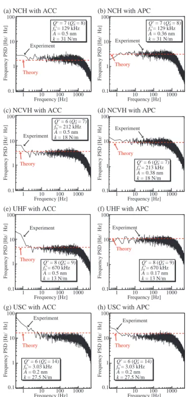
4.1.2. Photothermal excitation with ACC and APC drivers In this study, we found an important problem of the photothermal excitation method that prevents the stable operation of FM-AFM with a small cantilever. Figure 4 shows frequency spectral density (n

) distribution measured in water. The laser diode used for the cantilever excitation was driven by an automatic power constant (APC) or automatic current constant (ACC) circuit. The solid lines show the experimentally measured spectra while the dotted lines show the frequency spectral density (n

) corresponding to the noise arising from the thermal Brownian motion of the cantilever. The values of n

were calculated by following equation[3, 38].

n

=

s

k

T f

πkQ

A

, (11)

where Q

is the apparent Q-factor calculated from the slope of a phase versus frequency curve obtained in liquid. The bandwidth of the PLL was set at 1 kHz. Thus, n

shows a sharp decrease around 1 kHz.

From 10 Hz to 1 kHz, all the spectra in figure 4 show good agreement with n

.

However, the spectra obtained with the ACC driver show an increase from n

at

the frequency range below 10 Hz. This low frequency noise becomes more and more

prominent with reducing the cantilever size. In this study, we found that this low

frequency noise can be greatly suppressed by replacing the ACC driver with an APC

driver. For the NCH, NCVH and UHF cantilevers, this improvement was effective

0.1 100

1 10 100 1000

10

FrequencyPSD[Hz/√Hz]

Frequency [Hz]

(c) NCVH with ACC

0.1 1 100

1 10 100 1000

10

FrequencyPSD[Hz/√Hz]

Frequency [Hz]

(d) NCVH with APC

0.1 1 100

1 10 100 1000

10

FrequencyPSD[Hz/√Hz]

Frequency [Hz]

Theory Experiment

Theory

Theory Theory

Theory

Theory

Theory

Theory Experiment

Experiment

Experiment Experiment

Q^*= 7 (Qd= 8) f₀= 129 kHz A= 0.5 nm k= 31 N/m

Q^*= 6 (Q_d= 7) f₀= 212 kHz A= 0.5 nm k= 18 N/m

Q^*= 8 (Qd= 9) f₀= 670 kHz A= 0.5 nm k= 13 N/m

Q^*= 6 (Qd= 14) f₀= 3.03 kHz A= 0.2 nm k= 27.5 N/m

Q^*= 6 (Qd= 14) f₀= 3.03 kHz A= 0.2 nm k= 27.5 N/m

Q^*= 8 (Qd= 9) f₀= 670 kHz A= 0.17 nm k= 13 N/m Q^*= 6 (Qd= 7) f₀= 213 kHz A= 0.38 nm k= 18 N/m

Q^*= 7 (Qd= 8) f₀= 129 kHz A= 0.36 nm k= 31 N/m Experiment

Experiment

Experiment

(a) NCH with ACC

0.1 1 100

1 10 100 1000

10

FrequencyPSD[Hz/√Hz]

Frequency [Hz]

(b) NCH with APC

0.1 100

1 10 100 1000

10

FrequencyPSD[Hz/√Hz]

Frequency [Hz]

(e) UHF with ACC

0.1 1 100

1 10 100 1000

10

FrequencyPSD[Hz/√Hz]

Frequency [Hz]

(f) UHF with APC

0.1 100

1 10 100 1000

10

FrequencyPSD[Hz/√Hz]

Frequency [Hz]

(g) USC with ACC

0.1 1 1

1 1

100

1 10 100 1000

10

FrequencyPSD[Hz/√Hz]

Frequency [Hz]

(h) USC with APC

*

* *

*

*

*

*

*

*

*

*

*

* *

*

*

Figure 4. Frequency spectral density distributions measured in water. The solid lines show experimentally measured spectra while the dotted lines shownf Bcalculated from equation (11).

enough to allow stable operation of FM-AFM. For the USC cantilever, however, the low frequency noise still remains [figure 4(h)].

The improvement achieved by the APC driver suggests that the low frequency noise

is caused by the laser power fluctuation. However, we experimentally confirmed that the

averaged power of the excitation laser beam driven by the ACC driver is as stable as that by the APC driver. In the photothermal excitation, the delay caused by the thermal expansion should be dependent on the laser beam position rather than the power of it.

Thus, the observed instability is more likely to be caused by the pointing instability of the laser beam.

4 3 2 1 0

0 2 4 6 8 10

Time [min]

FrequencyShift[kHz]

-1 -2

Q^*= 8 (Q_d= 16) f₀= 3.09 MHz A= 0.24 nm k= 27.5 N/m Q^*= 8 (Q_d= 16)

f₀= 3.09 MHz A= 0.1 nm k= 27.5 N/m

Theory

Experiment APC

ACC+TEC

0.1 100

1 10 100 1000

10

1

FrequencyPSD[Hz/√Hz]a

Frequency [Hz]

(b) (a)

(c)

*

*

*

*

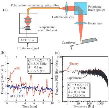
Cantilever Collimation lens Polarization-maintaining optical fiber

ACC driver Excitation signal

LD Temperature

controlled unit

Focus lens Polarizing beam splitter

Figure 5. (a) Schematic drawing of the setup for the photothermal excitation using PMF and ACC+TEC driver. (b) Time dependence of the frequency shift signal measured with the APC and ACC+TEC drivers. (c) Frequency spectral density distribution measured with the ACC+TEC driver. The measurements were performed in water using the USC cantilever.

4.1.3. Photothermal excitation with ACC+TEC driver To improve the pointing stability of the laser beam, we have made several modifications as shown in figure 5(a).

The laser diode module driven by an ACC driver was integrated into a temperature controlled (TEC) unit. In addition, the laser beam from the unit is transmitted through a polarization-maintaining optical fiber (PMF), which is known to be more immune to the mechanical vibration and temperature drift than a standard single mode fiber. The output from the PMF fiber is irradiated to the backside of a cantilever through a collimation lens, a polarizing beam splitter and a focus lens. Owing to these modifications, the laser beam profile becomes closer to a Gaussian profile and the pointing stability has been greatly improved.

Figure 5(b) shows time dependence of the frequency shift signal measured in water

with the APC and ACC+TEC drivers. The frequency shift signal measured with the

APC driver shows much larger fluctuation than that obtained with the ACC+TEC

driver. The result shows that the modifications that we made are effective to reduce

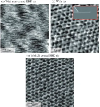
2 nm

(a) With non-coated EBD tip (b) With tip

(c) With Si-coated EBD tip

2 nm 1 nm

Figure 6. FM-AFM images of a cleaved mica surface obtained in PBS solution using USC cantilevers. (a) With non-coated tip (Q = 4.8,f0 = 2.7 MHz, ∆f = 27.8 kHz, A= 0.63 nm, 65 sec/frame). (b) Without tip (Q= 4.2,f0= 2.9 MHz, ∆f = 29.0 kHz, A= 0.31 nm, 65 sec/frame). The inset shows an SEM image of the USC cantilever obtained after the experiment. (c) With Si-coated tip (Q = 10, f0 = 3.1 MHz,

∆f = 1.64 kHz, A = 0.34 nm, 65 sec/frame). The thickness of the Si coat was 30 nm.

the low frequency noise. In fact, n

measured with the ACC+TEC driver [figure 5(c)]

shows good agreement with n

even at the frequency range less than 10 Hz.

We have not tried to use APC+TEC setup because of the following reason.

In general, it has been known that ACC+TEC provides better stability and noise performance than APC+TEC. In APC, noise from a laser beam and a monitor photodiode is fed back to the laser drive current. Thus, it tends to increase the noise compared to ACC. The main reason to use APC drive is to suppress the power fluctuation caused by the temperature drift of the laser diode. Therefore, as long as the temperature is well controlled with a TEC setup, the use of APC drive increases the output noise without improving the stability.

4.2. Weak interaction between EBD tip and surface

As the cantilever size is reduced, it becomes difficult to fabricate a sharp tip at its

end. In addition, the mass of the tip becomes non-negligible compared with that of the

cantilever body, leading to a decrease of f

. This partially cancels out the enhancement

of f

obtained by the reduction of the cantilever size. To solve this problem, the USC

cantilever is equipped with an EBD tip. Owing to the small mass, the increase of f

caused by the EBD tip is negligible.

However, in this study, we found great difficulties in using the EBD tip for an atomic-resolution imaging. Figure 6(a) shows an FM-AFM image of a cleaved mica surface obtained in phosphate buffered saline (PBS) solution by the USC cantilever with the EBD tip. Although the force detection was sensitive and the tip-sample distance regulation was stable, we were not able to obtain atomic-resolution images.

To gain insight into the influence of the EBD tip, we crashed the tip into the surface and removed it. The detachment of the tip from the cantilever was confirmed by the significant decrease of the Q factor during the imaging. In addition, it is also confirmed by the SEM image of the cantilever obtained after the experiment [inset in figure 6(b)].

After the tip crash, it suddenly became possible to obtain an atomic-resolution image as shown in figure 6(b). As the tip was completely removed from the cantilever, it is most likely that the edge of the cantilever worked as a tip during the imaging. These results suggest that the difficulty in obtaining an atomic-resolution image is not caused by the USC cantilever but by the EBD tip.

We observed such changes caused by the tip crash using two different USC cantilevers and confirmed the reproducibility. We also performed similar experiments on calcite surface in pure water and found that we were not able to obtain clear atomic- resolution images on this surface either. This result suggests that the problem is not specific to a mica surface but is more general.

A surface consisting of carbon atoms, such as highly oriented pyrolytic graphite (HOPG) surface, is known to be relatively inert and hence difficult to image by FM- AFM. Thus, the interaction between the carbon EBD tip and sample surface should be relatively weak. This accounts for the difficulty in obtaining an atomic-resolution image by the EBD tip. To overcome this problem, we coated an EBD tip with Si by sputtering method (thickness: 30 nm). With the Si coated EBD tip, we were able to obtain a clear atomic-resolution image of mica as shown in figure 6(c). The result shows that the Si coating makes it possible to obtain atomic-resolution images even with a carbon EBD tip.

According to the manufacturer and our SEM experiments, the sharpness of the tip is almost the same for all the cantilevers including the USC cantilever ( ≈ 10 nm).

However, the Si coating with 30 nm thickness should increase the tip radius. For atomic- resolution imaging of a flat surface using small A, the increase of the tip radius hardly affects on the image quality as the short-range interaction between the tip front atom and surface topmost atom predominantly contributes to the frequency shift. However, the increase of the tip radius may increase the tip artifact if the tip is scanned on a surface having nanoscale corrugations.

For the oscillation amplitude, it has been experimentally and theoretically shown

that the optimal value roughly corresponds to the interaction length of the force to be

detected[39]. In the case of atomic-scale imaging, the interaction length of atom-atom

interaction is approximately a few Angstroms. In the actual experiment, we adjust A

for optimizing the image quality and typically find that 0.2–0.3 nm is the optimal value.

This was also true of the experiments using the USC cantilever.

So far, several research groups (including us) have shown clear atomic-resolution images of mica in liquid[4, 7]. The image quality depends not only on the force sensitivity but also on other factors such as the tip apex, solution condition and measurement bandwidth. Thus, it is very difficult to quantitatively show the improvement in F

from the image quality. Therefore, we decided to make such quantitative discussions using force curve data as shown below.

5. Measurements of hydration forces

To experimentally confirm the improvement in F

, we measured ∆f versus distance curves on mica in PBS solution using NCH and USC cantilevers [figures 7(a) and 7(b)].

The both ∆f curves show an oscillatory profile with a peak spacing of 0.3–0.4 nm. Such an oscillatory force has been attributed to the interaction between a tip and hydration layers formed on a mica surface[4, 40].

The ∆f curves are smoothed by averaging ten adjacent data points and are converted to force versus distance curves [figures 7(c) and 7(d)] using the formula reported by Sader and Jarvis[41]. The obtained force curves show similar values. For example, the difference between the largest peak and valley in the force curves is 0.17 and 0.20 nN for the NCH and USC cantilevers, respectively. In addition to these values, some of the physical quantities used in the following discussions are summarized in table 3.

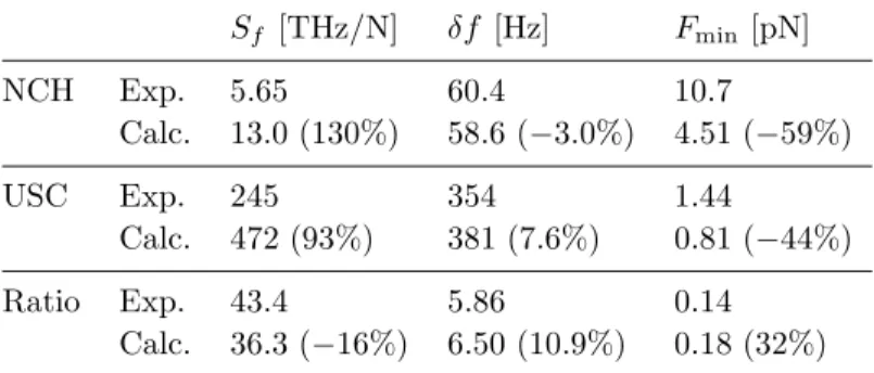
Table 3. Experimentally measured and theoretically calculated values ofSf, δf and Fmin. The experimental values were obtained by analyzing the data shown in figure 7.

The theoretical values were calculated from the cantilever parameters and equations (12), (11) and (10). The ratio in the table denotes the ratio of the values for the USC cantilever devided by those for the NCH cantilever. Figures in the parentheses show errors in the calculated values with respect to the measured ones.

Sf [THz/N] δf [Hz] Fmin[pN]

NCH Exp. 5.65 60.4 10.7

Calc. 13.0 (130%) 58.6 (−3.0%) 4.51 (−59%)

USC Exp. 245 354 1.44

Calc. 472 (93%) 381 (7.6%) 0.81 (−44%)

Ratio Exp. 43.4 5.86 0.14

Calc. 36.3 (−16%) 6.50 (10.9%) 0.18 (32%)

In contrast to the quantitative agreement in the force value, the ∆f curves show significantly different values. For example, the difference between the largest peak and valley in the ∆f curves are 960 Hz and 49 kHz for the NCH and USC cantilevers, respectively. These ∆f values should respectively correspond to 0.17 and 0.20 nN force.

Thus, the force sensitivity (S

) obtained by the NCH and USC cantilevers is 5.65 and

Distance [nm]

FrequencyShift[kHz]

-1.00 -0.5 0 0.5 1.0 1.5

0.5 1.0 1.5 2.0 2.5 (a) Frequency shift curve (NCH)

Distance [nm]

FrequencyShift[kHz]

-400 -20 20 0 40 60

0.5 1.0 1.5 2.0 49 kHz 960 Hz

Raw data

0.17 nN

2.5 (b) Frequency shift curve (USC)

Distance [nm]

Force[nN]

-0.20 -0.1 0 0.1 0.2

Force[nN]

-0.2 -0.1 0 0.1 0.2

0.5 1.0 1.5 2.0 2.5 (c) Force curve (NCH)

Distance [nm]

0 0.5 1.0 1.5 2.0 2.5 (d) Force curve (USC)

Frequency [Hz]

FSD[Hz/√Hz]

10⁰ 10^-1 10⁰ 10¹ 10² 10³

10⁰ 10¹ 10² 10³ 10⁴

10¹ 10² 10³ 10⁰ 10¹ 10² 10³

Frequency [Hz]

FSD[Hz/√Hz]

(e) Frequency spectral density (NCH) (f) Frequency spectral density (USC) 0.20 nN Smoothed

Thermal

Experiment Thermal

Experiment Raw data Smoothed

Figure 7.(a), (b) ∆fversus distance curves obtained with NCH and USC cantilevers.

The black lines show raw data (sampling rate: 2 kHz, tip velocity: 1 nm/s,B = 100 Hz). The smoothed curves are obtained by averaging ten adjacent data points (red lines in color). A = 0.112 nm, k = 52.1 N/m, f₀^∗ = 149.8 kHz and Q^∗ = Q^∗_d = 8.8 for the NCH cantilever. A= 0.136 nm, k= 24.0 N/m, f₀^∗= 3.08 MHz,Q^∗= 6.3 and Q^∗_d= 15 for the USC cantilever. Note that ∆f values are multiplied by a correction factorQ^∗_d/Q^∗ for compensating the error caused by the phase delay in the cantilever excitation loop[38]. (c), (d) The smoothed curves are converted to force versus distance curves using the formula reported by Sader and Jarvis. (e), (f) The frequency spectral density distributions of the ∆f versus distance curves (raw data). The dotted lines correspond to n_{f B} values calculated from equation (11). Note that these calculated values are multiplied by a correction factorp

Q^∗_d/Q^∗for the same reason as described above.

245 THz/N, respectively. The result shows that S

is enhanced by 43 times using a small cantilever.

Equation (10) describing F

is obtained by taking the ratio of n

divided by S

. While n

is given by equation (11), S

is given by

S

= f

2kA . (12)

Equation (11) is valid for any oscillation amplitude while equation (12) is valid only when

A is small enough to consider the force gradient to be constant (i.e. small amplitude

approximation). In this experiment, A ( ≈ 0.1 nm) is comparable to the length scale of

the force variation. Thus, the small amplitude approximation should give some error in the estimation of S

. Here, we estimate this error and discuss the validity of the discussions made in this paper.

From equation (12), S

obtained with the NCH and USC cantilevers are calculated to be 13.0 and 472 THz/N, respectively. Compared with the experimentally measured values, the calculated values contain 130% and 93% errors for the NCH and USC cantilevers, respectively. Although these errors are not necessarily small, they are acceptable for order estimation.

Compared with the S

values, the relative improvement in S

can be more accurately estimated. This is because S

is proportional to f

/k not only in equation (12) but also in the accurate formula describing S

[42]. In fact, the improvement in S

calculated from equation (12) is 36.3 times, which contains − 16% error compared with the experimentally measured value. This error is small enough to support the discussions made in the paper.

For quantitative estimation of noise in the force curves, we have converted the ∆f curves (raw data) to frequency spectral density (FSD) distributions [figures 7(e) and 7(f)]. The FSD spectrum obtained with the USC cantilever [figure 7(f)] shows a clear peak around 3 Hz as indicated by an arrow. As the tip velocity during the measurement was 1 nm/s, this peak corresponds to the oscillatory behavior of the ∆f curves with a peak spacing of approximately 0.3 nm. In the FSD spectrum obtained with the NCH cantilever [figure 7(e)], such a peak is barely recognized due to the large noise. These results show that the signal-to-noise ratio (SNR) in the ∆f curve is significanly improved by using the USC cantilever. Owing to the high SNR in the ∆f curve obtained by the USC cantilever, we can recognize the small peak corresponding to the third hydration layer [figure 7(b)]. However, it is not visible in the curve obtained by the NCH cantilever due to the low SNR [figure 7(a)].

We have calculated n

from equation (11) for the NCH and USC cantilevers and obtained 5.86 and 44.7 Hz/

√

Hz, respectively. For the both FSD spectra, the calculated values (dotted lines) agree with the floor noise level. We estimated the floor noise level by averaging the FSD values at the frequency range from 10 to 100 Hz and obtained 6.04 and 35.4 Hz/

√

Hz for the NCH and USC cantilevers. From these n

values and B = 100 Hz, we calculated total frequency noise (δf ) and summarized in table 3. The table shows that the error contained in the calculated δf values is less than ± 10%, which is within the acceptable range to support the discussions made in this paper.

From the experientally measured S

and δf values, we have calculated F

and obtained 10.7 and 1.44 pN for the NCH and USC cantilevers, respectively. The result shows that F

is improved by 7.1 times using a small cantilever. From equation (10), this improvement was estimated to be 5.6 times, which contains 32% error compared with the experimentally obtained value. This error is also small enough to support the discussions made in this paper.

In this experiment, we have measured hydration forces and confirmed the

improvement in F

obtained by the small cantilever. Among various force components,

hydration force has one of the shortest interaction length ( ≈ 0.3 nm). Even for such a severe condition, the F

value calculated with the small amplitude approximation was comparable to the experimentally obtained one. Therefore, the same discussion should hold for most of the other force components.

6. Conclusions

In this study, we have investigated the FM-AFM performance obtained by various cantilevers with different dimensions from theoretical and experimental aspects. We experimentally confirmed that the smaller cantilever actually provides the lower F

owing to the higher f

as theoretically expected. While this rule is always valid far from the surface, it can fail near the surface due to the Q damping caused by the squeeze film effect. To avoid this, the tip height should be sufficiently long compared with the cantilever width.

We have revealed two important issues to be overcome for applying a small cantilever to atomic-resolution FM-AFM imaging. The stable excitation of a small cantilever requires much higher pointing stability of the excitation laser beam than that for a long cantilever. We have presented a way to satisfy this requirement using a TEC laser diode module driven with an ACC driver and a polarization-maintaining optical fiber. We also found that atomic-resolution imaging with a carbon EBD tip is very difficult due to the weak interaction between the carbon tip and sample surface.

However, we have shown that the tip-sample interaction can be greatly enhanced by coating the EBD tip with Si. Finally, using the improved photothermal excitation setup and Si-coated EBD tip, we have demonstrated stable atomic-resolution imaging of mica in liquid by a small cantilever with a megahertz-order resonance frequency. In addition, we have experimentally demonstrated the improvement in F

obtained by the small cantilever in the measurements of oscillatory hydration forces.

So far, F

obtained by FM-AFM in liquid has been just as much as required

for the atomic-resolution imaging. In this study, we experimentally demonstrated

seven-fold improvement in F

obtained by the small cantilever. This improvement

should provide enough margin to secure reproducibility, reliability and efficiency in the

atomic-scale applications. In addition, the improvement in F

should also improve

the performance of surface property measurement techniques combined with FM-AFM,

where their resolution has still been limited by the force sensitivity. Furthermore, the

sevel-fold improvement in F

corresponds to 49-fold improvement in the operation

speed. So far, an atomic-resolution image is typically obtained in 50–100 sec with a

standard cantilever. Thus, we should be able to obtain the same image in 1–2 sec

with a small cantilever. Therefore, the achievements obtained in this study should also

contribute to the development of high-speed FM-AFM.

Acknowledgments

This work was supported by KAKENHI (21681018), Japan Society for the Promotion of Science and PRESTO, Japan Science and Technology Agency.

References

[1] T. R. Albrecht, P. Gr¨utter, D. Horne, and D. Ruger. J. Appl. Phys., 69:668, 1991.

[2] S. Morita, R. Wiesendanger, and E. Meyer, editors. Noncontact Atomic Force Microscopy (Nanoscience and Technology). Springer Verlag, 2002.

[3] T. Fukuma, M. Kimura, K. Kobayashi, K. Matsushige, and H. Yamada. Rev. Sci. Instrum., 76:053704, 2005.

[4] T. Fukuma, K. Kobayashi, K. Matsushige, and H. Yamada. Appl. Phys. Lett., 87:034101, 2005.

[5] K.-I. Umeda and K.-I. Fukui. Langmuir, 26:9104, 2010.

[6] K.-I. Umeda and K.-I. Fukui. J. Vac. Sci. Technol. B, 28:C4D40, 2010.

[7] B. W. Hoogenboom, H. J. Hug, Y. Pellmont, S. Martin, P. L. T. M. Frederix, D. Fotiadis, and A. Engel. Appl. Phys. Lett., 88:193109, 2006.

[8] M. Higgins, M. Polcik, T. Fukuma, J. Sader, Y. Nakayama, and S. P. Jarvis. Biophys. J., 91:2532, 2006.

[9] T. Fukuma, M. J. Higgins, and S. P. Jarvis. Biophys. J., 92:3603, 2007.

[10] T. Fukuma, M. J. Higgins, and S. P. Jarvis. Phys. Rev. Lett., 98:106101, 2007.

[11] T. Fukuma, A. S. Mostaert, and S. P. Jarvis. Nanotechnology, 19:384010, 2008.

[12] H. Asakawa and T. Fukuma. Nanotechnology, 20:264008, 2009.

[13] H. Yamada, K. Kobayashi, T. Fukuma, Y. Hirata, T. Kajita, and K. Matsushige. Appl. Phys.

Express, 2:095007, 2009.

[14] K. Nagashima, M. Abe, S. Morita, N. Oyabu, K. Kobayashi, H. Yamada, M. Ohta, R. Kokawa, R. Murai, H. Matsumura, H. Adachi, K. Takano, and S. Murakami. J. Vac. Sci. Technol. B, 28:C4C11, 2010.

[15] H. Asakawa, K. Ikegami, M. Setou, N. Watanabe, M. Tsukada, and T. Fukuma. Biophys. J., 101:1270, 2011.

[16] M. B. Viani, T. E. Sch¨affer, A. Chand, M. Rief, H. E. Gaub, and P. K. Hansma. J. Appl. Phys., 86:2258, 1999.

[17] S. Hosaka, K. Etoh, A. Kikukawa, H. Koyanagi, and K. Itoh. Microelectronic Engineering, 46:109, 1999.

[18] J. L. Yang, M. Despont, U. Drechsler, B. W. Hoogenboom, P. L. T. M. Frederix, S. Martin, A. Engel, P. Vettiger, and H. J. Hug. Appl. Phys. Lett., 86:134101, 2005.

[19] T. E. Sch¨affer and P. K. Hansma. J. Appl. Phys., 84:4661, 1998.

[20] S. Hosaka, K. Etoh, A. Kikukawa, and H. Koyanagi. J. Vac. Sci. Technol. B, 18:94, 1999.

[21] B. W. Hoogenboom, P. L. T. M. Frederix, J. L. Yang, S. Martin, Y. Pellmont, M. Steinacher, S. Z¨ach, E. Langenbach, and H.-J. Heimbeck. Appl. Phys. Lett., 86:074101, 2005.

[22] S. Kawai, D. Kobayashi, S.-I. Kitamura, S. Meguro, and H. Kawakatsu. Rev. Sci. Instrum., 76:083703, 2005.

[23] R. Enning, D. Ziegler, A. Nievergelt, K. Venkataramani, and A. Stemmer. Rev. Sci. Instrum., 80:043705, 2011.

[24] G. T. Paloczi, B. L. Smith, P. K. Hansma, D. A. Walters, and M. A. Wendman. Appl. Phys. Lett., 73:1658, 1998.

[25] T. Ando, N. Kodera, E. Takai, D. Maruyama, K. Saito, and A. Toda. Proc. Natl. Acad. Sci. USA, 98:12468, 2001.

[26] C. P. Green and J. E. Sader. J. Appl. Phys., 98:114913, 2005.

[27] S. Basak, A. Raman, and S. V. Garimella. J. Appl. Phys., 99:114906, 2006.

[28] R. C. Tung, A. Jana, and A. Raman. J. Appl. Phys., 104:114905, 2008.

[29] T. Fukuma and S. P. Jarvis. Rev. Sci. Instrum., 77:043701, 2006.

[30] T. Fukuma. Rev. Sci. Instrum., 80:023707, 2009.

[31] S. Morita, R. Wiesendanger, and F. J. Giessibl, editors. Noncontact Atomic Force Microscopy Volume 2 (Nanoscience and Technology). Springer Verlag, 2009.

[32] J. E. Sader. J. Appl. Phys., 84:64, 1998.

[33] T. Naik, E. K. Longmire, and S. C. Mantell. Sens. Actuators, 102:240, 2003.

[34] A. Maali, C. Hurth, R. Boisgard, C. Jai, T. Cohen-Bouhacina, and J.-P. Ami´e. J. Appl. Phys., 97:074907, 2005.

[35] Y. Martin, C. C. Williams, and H. K. Wickramasinghe. J. Appl. Phys., 61:4723, 1987.

[36] S. P. Jarvis, A. Oral, T. P. Weihs, and J. B. Pethica. Rev. Sci. Instrum., 64:3515, 1993.

[37] N. Umeda, S. Ishizaki, and H. Uwai. J. Vac. Sci. Technol. B, 9:1318, 1991.

[38] T. Fukuma. Sci. Technol. Adv. Mater., 11:033003, 2010.

[39] F. J. Giessibl, H. Bielefeldt, S. Hembacher, and J. Mannhart. Appl. Surf. Sci., 140:352, 1999.

[40] T. Fukuma, Y. Ueda, S. Yoshioka, and H. Asakawa. Phys. Rev. Lett., 104:016101, 2010.

[41] J. E. Sader and S. P. Jarvis. Appl. Phys. Lett., 84:1801, 2004.

[42] F. J. Giessibl. Appl. Phys. Lett., 78:123, 2001.