Measurements of Mass Flux and Concentration in Supersonic Air/Helium Mixing by Hot-Wire Anemometry

Proceedings of the 40th JAXA Workshop on “Investigation and Control of Boundary-Layer Transition” 　

Measurements of Mass Flux and Concentration in Supersonic Air/Helium Mixing by Hot-Wire Anemometry

Akira KONDO ^* , Shoji SAKAUE ^* and Takakage ARAI ^*

* Graduate school of Aerospace Engineering Osaka Prefecture University, Sakai, Osaka, Japan

ABSTRACT

In the present study we made efforts to realize a measurement method of mass flux and concentration in supersonic air/helium flow in order to clarify the mixing process. The measuring equipment, which was used for measuring the fluctuations of mass flux and concentration, is consisted of a double-hot-wire probe and CVA (Constant Voltage Anemometer) circuit with 500 kHz bandwidth. The distance between two wires of double-hot-wire probe was 0.16 mm. By using the same material as the hot wire, the correlation coefficient between each hot wire output in Mach 2.4 supersonic flow with the pair of streamwise vortices was about 0.9. Therefore, we confirmed that the flows captured by two wires were almost the same and our device can capture the coherent structure up to 1 mm in Mach 2.4 supersonic flow. When we use the two kinds of wires with the different responses to the variations of mass flux and helium concentration, we can find the air/helium mixing flow field using the calibration maps of each wires. In the present study, we used the two tungsten wires with 5 Pm and 3.1 Pm in diameter as the double-hot-wire probe and measure the mean mass flux and helium concentration in supersonic air/helium mixing layer in order to improve our measuring method.

Key Words: Supersonic Mixing, Mixing Enhancement, Hot-Wire Measurement, CVA (Constant Voltage Anemometer)

1. Introduction

The measurement of instantaneous mixing process in supersonic flow is great important on supersonic mixing enhancement such as development of scramjet engine. The quantitative measurement methods for fluctuating mass flux and concentration have been proposed by Xillo et al. ¹⁾ and Arai et al. ²⁾ . But they have not been established yet because of the lack of time resolution. The purpose of this study is to establish the instantaneous quantitative measurement method for mass flux and concentration of mixing flow filed.

2. Experimental apparatus and procedure

The principle of our measurement method is almost the same method that Harion et al. ³⁾ have established in subsonic flow. Our device is consisted of double-hot-wire probe, as shown in Fig. 1, and CVA (Constant Voltage Anemometer) circuit with 500 kHz bandwidth. The double-hot-wire probe needs two kinds of wires with different characteristics of heat transfer. The heat balances of each wire are written as follows,

^{ޓޓ ( 1 , 2 )}

2

A c B c u i R

R R

V

i ai i

wi wi

wi

U (1)

where V w is the voltage across the hot wire, R w is the resistance of the hot wire at the operating temperature, R a is the resistance of the unheated wire at ambient temperature, U _u is the mass flux, and c is the concentration of the fuel gas. In this study, we use helium gas as pseudo fuel. Left side of the eq. (1) indicates the power dissipation ratio (PDR) of the hot wire. Eliminating the square root of the mass flux from eq. (1), we obtain the following iso-concentration equation.

c ^{A c} B

c c B A c PDR B

c

PDR B

2 1 1 2 2

1

1

(2)

From eq. (2), we can detect the helium concentration c . Substituting the obtained c into eq. (1), mass flux U u is obtained.

Flow

Hot Wire 2 ( I 3.1 Pm Tungsten) 0.16mm

Hot Wire 1 ( I 5.0 Pm Tungsten) Flow

Hot Wire 2 ( I 3.1 Pm Tungsten) 0.16mm

0.16mm

Hot Wire 1 ( I 5.0 Pm Tungsten)

Fig. 1 Double-hot-wire probe.

3. Problems of the measurement method

There are three problems in our measurement method for instantaneous mixing process in supersonic flow, that is, calibration, spatial resolution and thermal lag of hot wire response. In order to resolve these problems, we carried out the following experiments.

3.1 Calibration method

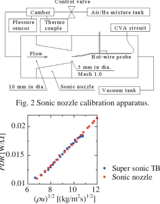
The coefficients A and B in eq. (1) are determined by the hot wire calibration for mass flux U u and concentration c . It is desirable that the hot wire is calibrated in the wind tunnel in which the measurements are conducted and for the wide variations of mass flux and concentration by as small amount of mixed gas as possible. Thus, we used the sonic nozzle calibration apparatus as shown in Fig. 2.

Air/helium mixed gas is blown down through the circular convergent nozzle whose exit diameter is 5 mm, and the hot wire is calibrated at the nozzle exit where the speed of mixed gas reaches Mach 1. By using the sonic nozzle apparatus, we can calibrate the hot wire for the wide variations of mass flux by the small amount of the mixed gas. However, we must confirm that the calibration results can be applied to the measurements in supersonic flow. Figure 3

This document is provided by JAXA.

6 JAXA Special Publication　JAXA-SP-07-06E

shows the comparison between the calibration results by using the sonic nozzle and in the supersonic turbulent boundary layer at Mach 2.4. As seen from Fig. 3, both results are in good agreement and the correlation coefficient is 0.997. Thus, we can conclude that the calibration results of the sonic nozzle can be applied to the measurements in supersonic flow.

Fig. 2 Sonic nozzle calibration apparatus.

Super sonic TBL Sonic nozzle

PD R [ W / : ]

( U _u ) ^1/2 [(kg/m ² s) ^1/2 ]

6 8 10 12

0.01 0.015

0.02

Fig. 3 Calibration results in sonic flow and in Mach 2.4 supersonic turbulent boundary layer.

3.2 Spatial resolution

The each hot wire of the double-hot-wire probe can not measure at the same point due to its configuration.

Therefore, the distance between the hot wires must be minimized. So we made the double-hot-wire probe whose distance between each wire was 0.16 mm and length of the wires was 0.5 mm. To confirm similarity of the outputs of the each hot wire, we measured the correlation coefficient between the each hot wire output in Mach 2.4 supersonic flow with two pairs of counter rotating streamwise vortices as shown in Fig. 4. Figure 5 shows instantaneous schlieren photograph of the flow field. The hot wire measurements were done at x = 100 mm, 2 mm ” y ” 14 mm, z = 15 mm. At x = 100 mm, the streamwise vortices grew up to y = 13 mm and the reflected shock wave passed at y = 5 mm. Figure 6 shows the correlation coefficients between the each hot wire output by using the same material. As seen from Fig.

6, the correlation coefficients at 5 mm ” y ” 13 mm were about 0.9. Thus, the flows captured by the two wires were almost the same and the flow structures in this region were larger than that in the near wall region. In other words, spatial resolution of our measurement method becomes the sensor size of the double-hot-wire probe 0.5 mm ˜ 0.16 mm.

(b) (a)

Flow

Flow x

z

y y

z x

Streamwise vortex

(b) (a)

Flow

Flow x

z

y y

z x

Streamwise vortex

Fig. 4 Schematic of test section and coordinate system (a) overhead view (b) cross section: circular lines

indicate streamwise vortices.

10

100

60 80 120

0 x [mm]

y [mm]

K.E.

10

100

60 80 120

0 x [mm]

y [mm]

K.E.

100

60 80 120

0 x [mm]

y [mm]

K.E.

K.E.

Fig. 5 Instantaneous schlieren photograph of Mach 2.4 supersonic flow with streamwise vortices.

Correlation [-]

y [ m m ]

0 0 0.2 0.4 0.6 0.8 1 3

6 9 12 15

Fig. 6 Correlation coefficients between each hot-wire output.

3.3 Compensation for the lag of hot-wire

The hot wire has the heat inertia, so that the response of the hot wire delays to the fluctuations of the flow. In addition, the time constant of the hot wire response changes according to the flow condition.

Thus, the thermal lags of the each hot wire must be compensated by the software processing method ⁴⁾ .

It is well known that the resistance of the hot wire depends on temperature,

R w = R ref [1 + D ( T w í T ref )] (3) and the time constant M of the hot wire by using the basic CVA circuit is written as follows,

2

1 1

2 _{ref w}

w w

w

R I C a

M a ˜ ˜

D (4)

where a w is the over heat ratio, C w is the heat capacity of the hot wire, I w is the current through the wire and R ref is the resistance of the unheated wire at reference temperature T ref . C w / D R ref is the constant value peculiar to the each wire, a w and I w can be determined by measurement. Therefore, the time constant of the hot wire can be determined if C w / D _{R ref} is known.

Figure 7 shows the typical response of the hot wire when a square wave is injected through input terminal of the CVA circuit. From the results as shown in Fig.

7, the time constant of the wire is determined as the time taken to reach the 63.2% of the final value, and C w / D R ref is known from eq. (4).

This document is provided by JAXA.

Proceedings of the 40th JAXA Workshop on “Investigation and Control of Boundary-Layer Transition” 　7

Time [s] Time [s]

V

[V] V

[V]

0 0.002

3.9 4 4.1

0.632 0 1

M

0 0.002

-7 -6.8 -6.6

Fig. 7 Inputted step wave and first order lag response waveform of hot wire.

4. Measurements in mixing layer

4.1 Calibration for concentration and mass flux In the present study, two kinds of tungsten wires were used for the double-hot-wire probe, their diameter were 5 Pm (W5) and 3.1 Pm (W3.1), respectively. Figure 8 shows the calibration results of the each wire. From these results, the coefficients A and B in eq. (1) were ditermined as cubic functions of helium concentration, as shown in Fig. 9. Figure 10 shows the calibration map of eq. (2) by using A and B in Fig. 9.

In order to estimate the error included in our measurement method, Fig. 11 shows the comparison between the measurement value and the actual value of mass flux and helium concentration. Here, the measurement value means the value calculated from PDR of each hot wire by using the calibration map as shown in Fig. 10. As seen from Fig. 11, it is found that the error in this method was less than ±10%, except for the small PDR region where the iso-concentration lines were close to each other.

(U u)

[(kg/m

s)

] PD R

( W 5 ) [W / : ]

He 0 %, He 20 %, He 40 %, He 60 %, He 100 %

4 6 8 10

0.01 0.015 0.02 0.025

(U u)

[(kg/m

s)

] PD R

( W 3 .1 ) [W / : ]

4 6 8 10

0.002 0.004 0.006 0.008

Fig. 8 Calibration results for helium concentration and mass flux.

A ( c ),W5 A(c),W3.1 B ( c ),W5 B ( c ),W3.1

c [-]

A ( c ) [W / : ] B ( c ) [W / : (k g /m

s) ]

0 0.2 0.4 0.6 0.8 1 -0.01

-0.005 0 0.005

Fig. 9 A(c) and B(c) determined by Fig. 8: each line indicate cubic approximation for helium concentration.

PDR ₂ (W3.1) [W/:]

PD R 1 ( W 5 ) [W / : ]

He 0 % He 20 % He 40 % He 60 % He 80 % He 100 % 0.002 0.004 0.006 0.008

0.012 0.016 0.02 0.024 0.028

Fig. 10 Calibration map used for detecting helium concentration.

PDR

(W5) [W/:]

c

- c

[ % ]

He 0 %, He 20 %, He 40 %, He 60 %, He 100 % 0.01 0.015 0.02 0.025

-10 0 10 20 30 40

PDR

(W5) [W/:]

U u

- U u

[ k g /m

s]

0.01 0.015 0.02 0.025 -20

-10 0 10

Fig. 11 Difference between measurement value and actual value of helium concentration and mass flux.

4.2 Results and Discussions

In order to demonstrate the usefulness and to clarify the accuracy of our method, we applied our method to the measurement of two dimensional air/helium mixing layer as shown in Fig. 12. Air and helium flow, whose Mach number were 2.4 and 0.8 respectively, were separated by a thin splitter plate and the mixing layer was formed at the plate downstream. The length of the test section was 400 mm, the height was 35.5 mm and the width was 30 mm. Figure 13 shows the instantaneous schlieren photographs of the mixing layer just behind the splitter plate. The measurements were conducted at x = 30 mm and x = 100 mm, í4 mm ” y ” 10 mm and z = 15 mm.

M2.4 Air M0.8 He 18mm

35.5mm Mixing Layer

M2.4 Air M0.8 He 18mm

35.5mm Mixing Layer

Fig. 12 Schematic of the mixing layer.

Figure 14 shows the mass flux and the helium concentration profiles of the mixing layer. In these figures, blue lines indicate the profile at x = 30 mm, red lines are at x = 100 mm. At these stations, air and helium do mix only at the center region of the mixing layer as seen from the schlieren photographs shown in Fig. 13, so that the helium concentration must be zero at the upper side of the mixing layer and must be one at the lower side of the mixing layer.

This document is provided by JAXA.

JAXA Special Publication　JAXA-SP-07-06E

Fig. 13 Schlieren photographs of the mixing layer.

c [-]

y [ m m ]

x=30 mm, x=100 mm -0.2 0 0.2 0.4 0.6 0.8 1

-4 -2 0 2 4 6 8 10

U _u [kg/m ² s]

y [ m m ]

0 20 40 60 80100120 -4

-2 0 2 4 6 8 10

Fig. 14 Measurement results of helium concentration and mass flux in the mixing layer.

PDR ₂ (W3.1) [W/:]

PD R 1 ( W 5 ) [W / : ] x=30 mm x=100 mm He 0 % He 20 % He 40 % He 60 % He 80 % He 100 % y

Air

He

0.002 0.004 0.01

0.012 0.014 0.016 0.018 0.02

Fig. 15 Measurement results of the mixing layer plotted on the calibration map of Fig.10.

I 5 Pm, W, c =0 I 5 Pm, W, c=1 I 3.1 Pm, W, c =0 I 3.1 Pm, W, c =1 I 5 Pm, Pt, c =0 I 5 Pm, Pt, c=1 ( U _u ) ^1/2 [(kg/m ² s) ^1/2 ]

PD R [ W / : ]

4 6 8 10 12

0 0.01 0.02 0.03

Fig. 16 Calibration results of I 5 Pm and I 3.1 Pm tungsten wire and I 5 Pm platinum wire.

However, the results of the helium concentration were inconsistent, especially at the lower side of the mixing layer. Figure 15 plots the results of Fig. 14 on the calibration map of Fig. 10. In the lower side of the mixing layer, the power dissipation ratios of each hot wire were extremely small and the iso-concentration lines were close to each other as mentioned above.

Therefore, the results could not be estimated correctly in this region. However, this can be improved if we select the proper material as the hot wire. Figure 16 plots the calibration results of the platinum wire whose diameter was 5 Pm together with the calibration results of the two kinds of tungsten wires as shown in Fig. 8. As seen from Fig. 8, it is found that calibration results were changed by materials of hot wire. Therefore, by selecting proper wire materials, the intervals of the iso-concentration lines such as shown in Fig. 15 can be extended and the calibration map can be improved.

5. Conclusions

In the present study, we proposed simultaneous quantitation method of fluctuating mass flux and concentration. At first we resolve three problems in this method: calibration, spatial resolution and thermal lag of hot-wire response. Next, to demonstrate the usefulness of our method, we measured the air/helium mixing layer by using this method, and were able to obtain mass flux and helium concentration separately.

Acknowledgements

The present research was supported, in part, JSPS, Grant-in-Aid for Scientific Research, 1760694, 2005-2006.

References

1) O. C. Xillo, J. A. Schetz, W. F. Ng, and R. L.

Simpson, “A Sampling Probe for Fluctuating Concentration Measurement in Supersonic Flow,”

M. S. thesis, Virginia Polytechnic Institute and State University, Blacksburg, 1998.

2) T. Arai, K. Mizobata, R. Minato, N. Tanatugu, Y.

Mori, and T. Kudo, “Correlation between Fluctuations of Mass Flux and Hydrogen Concentration in Supersonic Mixing,”

AIAA-2005-323 AIAA/CIRA 13th International Space Planes and Hypersonics Systems and Technologies Conference, Capua, Italy, May 16-20, 2005.

3) J. L. Harion, M. Favre-Marinet, B. Camano, “An Improved Method for Measureing Velocity and Concentration by Thermo-Anemometry in Turbulent helium-air mixtures,” Experiments in Fluid, Vol.22, pp.174-182, 1996.

4) G. R. Sarma, “Transfer function analysis of the constant voltage anemometer,” Review of Scientific Instruments, Vol.69, Num.6, pp.2385-2391, 1998.

This document is provided by JAXA.