ATTA: AUTOMATIC TIME-SPAN TREE ANALYZER BASED ON EXTENDED GTTM

(1)

ATTA: AUTOMATIC TIME-SPAN TREE ANALYZER BASED ON EXTENDED GTTM

Masatoshi Hamanaka Keiji Hirata Satoshi Tojo PRESTO, Japan Science and

Technology Agency A.I.S.T. 1-1-1 Umezono,

Tsukuba, Ibaraki, Japan

[email protected]

NTT Communication Science Laboratories

2-4, Hikaridai, Seikacho, Kei- hanna Science City, Kyoto, Japan

[email protected]

Japan Advanced Institute of Science and Technoloty

1-1, Asahidai, Nomi, Ishikawa, Japan

[email protected]

ABSTRACT

This paper describes a music analyzing system called the automatic time-span tree analyzer (ATTA), which we have developed. The ATTA derives a time-span tree that assigns a hierarchy of 'structural importance' to the notes of a piece of music based on the generative theory of tonal music (GTTM). Although the time-span tree has been applied with music summarization and collabora- tive music creation systems, these systems use time-span trees manually analyzed by experts in musicology. Pre- vious systems based on GTTM cannot acquire a time- span tree without manual application of most of the rules, because GTTM does not resolve much of the ambiguity that exists with the application of the rules. To solve this problem, we propose a novel computational model of the GTTM that re-formalizes the rules with computer implementation. The main advantage of our approach is that we can introduce adjustable parameters, which en- ables us to assign priority to the rules. Our analyzer automatically acquires time-span trees by configuring the parameters that cover 26 rules out of 36 GTTM rules for constructing a time-span tree. Experimental results showed that after these parameters were tuned, our method outperformed a baseline performance. We hope to distribute the time-span tree as the content for various musical tasks, such as searching and arranging music.

Keywords: ATTA, Generative Theory of Tonal Music (GTTM), time-span tree, grouping structure, metrical structure, musical knowledge, knowledge acquisition.

1 INTRODUCTION

We propose a method for implementing a music theory called Generative Theory of Tonal Music (GTTM) [1].

It is difficult for those who are not musical experts to manipulate music, because commercial music se- quence software today only operates on the surface structure of music, such as the notes, rests, and chords.

Our goal is to create a system that will enable a musical novice to manipulate a piece of music, which is an ambiguous and subjective media, according to the user's intentions, by implementing the musical knowledge of mu- sicians. Our first step was to attempt to implement the GTTM, which analyses the meaning of a piece of music and interprets the implicit intentions of the composer.

Musical theory provides us with the methodologies for analyzing and transcribing musical knowledge, ex- periences, and skills from a musician's way of thinking.

Our concern is whether or not the concepts necessary for music analysis are sufficiently externalized in musical theory. We consider the GTTM to be the most promis- ing theory among the many that have been proposed [2–4], in terms of its ability to formalize musical knowledge, because the GTTM captures the aspects of the musical phenomena based on the Gestalt occurring in music and is presented with relatively rigid rules.

The time-span tree provides a summarization of a piece of music, which can be used as the representation of a search, by analyzing the results from the GTTM, re- sulting in a music retrieval system [5]. It can also be used for performance rendering [6-8] and reproducing music [9]. These systems enable users to manipulate music using a time-span tree, disregarding the surface structure of the music. However, the time-span trees in these systems need to be manually analyzed by experts in musicology.

The biggest problem with computer implementation of the GTTM is that musical theories, including GTTM, are ambiguous, because music interpretation is tacit and subjective. Beside that most of the musical theories are presented for humans, without taking into consideration computer logic. Attempts have been made to implement several rules of the GTTM, but when these rules conflict we could not adequately resolve the priority in multiple rules [10, 11]. On the other hand, the computer model of the GTTM [12] could produce a time-span tree, but it required manual application of most of the rules.

To overcome the ambiguity of the GTTM rules, we propose an extended GTTM that re-formalizes the rules and establishes an algorithm for acquiring a time- span tree by numerical expressions. In the expressions, we introduce adjustable parameters for controlling tacitness, ambiguity, and subjectiveness. The extended GTTM now covers 26 rules out of 36 GTTM rules for constructing a time-span tree. We implemented a time- span analyzer, called ATTA, based on the extended GTTM in Perl. User can acquire the time-span tree by Permission to make digital or hard copies of all or part of this

work for personal or classroom use is granted without fee pro- vided that copies are not made or distributed for profit or commercial advantage and that copies bear this notice and the full citation on the first page.

(2)

…

3a＾ 6 3a6 3a,6 This paper is organized in the following way. We

present the problem of applying GTTM rules in Sec- tion 2, propose extended GTTM in Section 3, describe the time-span analyzer and it’s examples in Section 4 and 5, and present experimental results and conclusion in Sections 6 and 7. Lastly, we provide in the appendix all the expressions to implement the GTTM analyzer.

2 INTRODUCTION OF GTTM AND ITS PROBLEMS

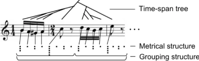
The GTTM is composed of four modules, each of which assigns a separate structural description to a listener’s understanding of a piece of music. These four modules output a grouping structure, a metrical structure, a time-span tree, and a prolongational tree, respectively (Figure 1).

…

・・・・・・・・・・・・・・・・

・・・・・・・・

・・・・・・・

Time-span tree

Metrical structure Grouping structure

Figure 1. Grouping structure, Metrical structure, and Time-span tree.

1 2 3 4 5 6 7 8 9 10 11 12 13 14

＾

＾＾＾

The grouping structure is intended to formalize the intuitive belief that tonal music is organized into groups that are in turn composed of subgroups. These groups are graphically presented as several levels of arcs below a music staff. The metrical structure describes the rhythmical hierarchy of the piece by identifying the po- sition of strong beats at the levels of a quarter note, half note, a measure, two measures, four measures, and so on. Strong beats are illustrated as several levels of dots below the musical staff. The time-span tree is a binary tree, which is a hierarchical structure describing the relative structural importance of notes that differentiate the essential parts of the melody from the ornamentation.

For example the left-hand side of Figure 2 depicts a simple melody and its tree. The time-span (designated as <--->) is represented by a single note, called a head, which is designated here as “C4”.

Abstracting Instantiating

C4 head C4

⊂ −

Figure 2. Subsumption relation of melodies.

There are two types of rules in GTTM, i.e., “well- formedness rules” and “preference rules”. Well- formedness rules are the necessary conditions for the assignment of a structure and the restrictions on the structures. When more than one structure satisfies the well-formedness rules, the preference rules indicate the superiority of one structure over another.

In this section, we specify the problems with the GTTM rules in terms of computer implementation.

2.1 Ambiguous concepts defining preference rules The GTTM uses some undefined words, causing ambiguities in the analysis. For example, the GTTM has rules for selecting proper structures when discovering similar melodies (called parallelism), but does not have the definition of similarity itself.

To solve this problem we attempted to formalize the cri- teria for deciding whether each rule is applicable or not.

2.2 Conflict between preference rules

The conflict between rules often occurs when applying the rules and results in ambiguities in the analysis because there is no strict order for applying the preference rules. Figure 3 shows a simple example of the conflict between the grouping preference rules (GPR). GPR3a (Register) is applied between notes 3 and 4 and GPR6 (Parallelism) is applied between notes 4 and 5. A boundary cannot be perceived at both 3-4 and 4-5, because GPR1 (alternative form) strongly prefers that note 4, by itself, cannot form a group.

To solve this problem we introduced adjustable parameters that enable us to control the strength of each rule.

Figure 3. Simple example of conflict between rules.

2.3 Few mentions to how to calculate hierarchical structures

The GTTM does not define a valid procedure for acquiring the hierarchical structure. It is not realistic to first make every structure satisfy the well-formedness rules and then select the optimal structure. For example, only a ten note score provides 185794560 (=9 !) kinds of time-span trees.

9　

2×

To solve this problem we developed an algorithm for acquiring the hierarchical structure, taking into consideration some of the examples in the GTTM.

2.4 Less precise explanation of feedback link

The GTTM has some feedback links from higher level structures to lower level ones, e.g. GPR7 (time-span and prolongational stability) prefers a grouping structure that results in a more stable time-span and/or prolonga- tion reductions. However, no detailed description and only a few examples are given.

3 EXTENDED GTTM

To overcome the problems with computer implementation of the GTTM, we propose a computational model of the GTTM called the extended GTTM, which covers 26 rules out of 36 GTTM rules for constructing time-span tree. The remaining 4 rules are for feedback links and another 6 rules are for homophony. In the current stage, we restrict the music structure to monophony to correctly evaluate the performance of each rule.

(3)

In this section we particularize our proposed exten- sion of the GTTM for computer implementation. The policies are equally applied to the three analyses, which are the grouping structure, metrical structure, and Time- span reduction analyses.

3.1 Re-formalization of rules

In order to deal with the preference rules on a computer, we have expressed the rules into numerical styles. Nu- meric descriptions of the rules allow to quantitatively combine the result of each rule application.

We expressed the degree of application of the rule as a numerical function Dirule which output 1 (applicable) or 0 (not applicable) if the rule is clearly applicable or not. For example, GPR2b (Attack-Point) states that a relatively greater interval of time between attack points initiates a grouping boundary that can be expressed as follows:

⎩⎨

⎧ < >

= ⁻ ⁺

lse e

ioi oi i and ioi oi i

D_i^GPR2b ⁱ ⁱ ⁱ ⁱ

0

1 ₁ ₁

, (1) i : transition of note

ioi i : inter onset intervals.

A numerical function Dirule outputs between 1 (applicable) and 0 (not applicable) if the rule is not clearly applicable or not. For example, time-span reduction preference rule 3a (TSRPR3a) that prefers that a higher melodic pitch is used as the head of a time-span can be expressed as follow:

j j TSRPR3 i

i pitch pitch

D = max , (2) i : head

pitch i : pitch (note number of MIDI).

3.2 Refinement of ambiguous concepts

As described above, the GTTM uses some undefined concepts that provide ambiguousness in analysis. The concepts are ambiguous, with no unique definition. For example, the concept of a similar melody has a lot of plausible definitions [13], but no best one.

Here, we attempted to formalize concepts based on the following two policies, which we esteem.

1) To define intuitionally and comprehensively.

2) Equipment adjustable parameters for control of the ambiguity.

3.2.1 Concept for symmetry

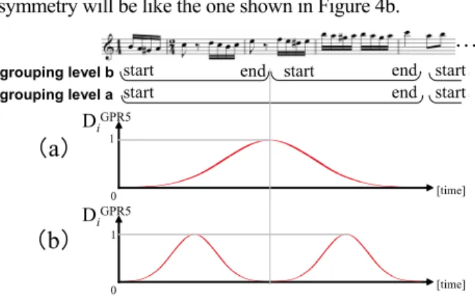
GPR5 is the rule for symmetry in a grouping structure. It prefers grouping analyses that most closely approach the ideal subdivision of groups into two parts of equal length.

We define the degree of symmetry DiGPR5 so that there is a preference to subdivide a group into two parts of equal length. Here, we use a normal distribution with the standard deviation σ as the degree of symmetry, as follows.

(3) where

start : start transition of group.

end : end transition of a group.

The σ is an adjustable parameter for a user to control the degree of symmetry. In Figure 4a is the degree of symmetry corresponding to grouping level a. If the next level boundary is found in the middle of the group by applying all grouping rules, the next grouping level’s the degree of symmetry will be like the one shown in Figure 4b.

start end start

grouping level a

start end start

grouping level b end start

D_i^GPR5

[time]

0

D_i^GPR5

[time]

0

（a）

（b）

…

1 1

Figure 4. Examples of symmetry level.

3.2.2 Concept for parallelism where

GPR6, MPR1, and TSRPR4 rules for parallelism are as follows.

GPR6: Where two or more segments of the music can be construed as parallel, they preferably form parallel parts of groups.

MPR1: Where two or more groups or parts of groups can be construed as parallel, they preferably form parallel metrical structures.

TSRPR4: If two of more time-spans can be construed as motivically and/or rhythmically parallel, preferably assign them parallel heads.

where

We formalized the concept of parallelism and defined the degree of parallel in each rule, because the target structures of the rules are different.

In GPR6, we focused on the parallelism of the segments. We introduced the degree of parallel for GPR6 DiGPR6, which indicates a high value at the start and end of the parallel part (Figure 5). The degree of parallel DiGPR6 was calculated by searching all the segments throughout the score. The length of the segments is from a beat to a half of the score by every beat.

GPR6 has three adjustable parameters for controlling the degree of parallel: Wr (priority to the same rhythm compared with the same register in parallel segments), Ws (priority to one end of a parallel segment compared with the start of the parallel segment), and Wl (priority to large parallel segments) (0≦Wr, Ws , Wl ≦1). By using these parameters, a user can easily find and con- figure the parallel segment.

D_i^GPR6

0 i

…

⎭

Figure 5. Example of the degree of parallel.

⎬⎫ σ2

⎩⎨

⎧ ⎟

⎠

⎜ ⎞

⎝

⎛ ∑ − ∑

−

= = =

GPR5 exp ^end 2 2

start

j j

i start

j j

i ioi ioi

D

(4)

In MPR1, we focused on the parallelism of beat in groups. We introduced the degree of parallel for MPR1 Di kMPR1, which is calculated by searching all the groups.

MPR1 has two adjustable parameters for controlling the degree of parallel: Wr (weight of priority of the same rhythm compared with the same register in parallel groups), and T^MPR1 (threshold that decides whether beat i and beat k are parallel (Di kMPR1= 1) or not (Di kMPR1= 0)).

In TSRPR4, we focused on the parallelism of time- spans, which are generated by grouping structure and metrical structure. We introduced the degree of parallel for TSRPR4 Di kTSRPR4, which is calculated by searching all the time-spans. TSRPR1 has no adjustable parameters for controlling the degree of parallel.

3.3 Resolving the preference rule confliction by pri- oritizing rules

We introduced adjustable parameters, S^rule, for controlling the strength of the GTTM rules. By using these parameters, we can acquire the local-level strength of boundary/beat/head. For example, as a result of applying the local-level grouping rules, we can acquire low-level grouping boundaries as weighted summations on the grouping rules results DiGPR and adjustable parameter S^GPR as follows:

⎟⎟⎠

⎜⎜ ⎞

⎝

⎛ ×

×

=

∑ ∑

= ′

=(2,2,3,3,3,3,6 ) ′ (2,2,3,3,3,3,6 )

max

d c b a b a j

j GPR j GPR i i

d c b a b a j

j GPR j GPR i

i D S D S

B .(4)

3.4 Top-down algorithm for calculating hierarchical structures

We introduced the top-down process for acquiring the structures. The hierarchal structure is constructed by calculating the local strength and choosing the next level structure.

- Acquisition of grouping structure

The grouping structure is constructed in the following way.

(1) First, consider the whole piece of music as a group.

(2) Then, calculate local-level boundary strengths and detect low-level boundaries.

(3) Next, select the strongest boundary and divide the group at the boundary.

(4) Finally, iterate (3) while the local boundaries are found at the group.

- Acquisition of metrical structure

The metrical structure is constructed in the following way.

(1) First, consider all the beats as a lowest (global) level metrical structure.

(2) Then, calculate the local-level metrical strength.

(3) Next, select the strongest metrical structure from possible structures.

(4) Finally, iterate (2) and (3) while the current structures have more than one beat.

- Acquisition of time-span tree

The time-span tree is constructed in the following way.

(1) First, consider all the notes as a head.

(2) Then, calculate the local-level head strength.

(3) Next, select the next level head from each time-span.

(4) Finally, iterate (2) and (3) while the time-span contains more than one head.

4 STRUCTURE OF ATTA

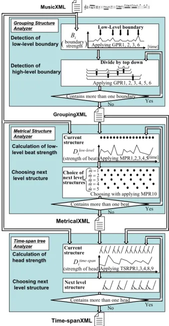
We implemented the extended GTTM described above on the computer that we call ATTA. Figure 6 is the over- view of the ATTA which consists of a grouping structure analyzer, a metrical structure analyzer, and a time- span tree analyzer. ATTA has three distinctive features, an XML-based data structure, its implemented in Perl, and has a Java-based GUI.

MusicXML

Low-Level boundary

[time]

boundary strength Detection of

low-level boundary

Detection of high-level boundary

GroupingXML

Divide by top down Applying GPR1, 2, 3, 6

Applying GPR1, 2, 3, 4, 5, 6

( )

B_i

Calculation of low- level beat strength

Choosing next level structure

MetricalXML

[time]

D_i^low-level

(strength of beat) Applying MPR1,2,3,4,5 Current

structure

Choice of next level structures

Choosing with applying MPR10 ˆ=1

mˆ=2 mˆ=3 mˆ=4 mˆ=5 m

No Yes Contains more than one beat

Calculation of head strength

Choosing next level structure

D_i^time-span

(strength of head)Applying TSRPR1,3,4,8,9 Current

structure

Next level structure

Time-spanXML No Yes Contains more than one head

No Yes Contains more than one boundary Grouping Structure

Grouping Structure Analyzer Analyzer

Metrical Structure Metrical Structure Analyzer Analyzer

Time Time--span tree span tree Analyzer Analyzer

Figure 6. Processing flow of ATTA.

4.1 XML based data structure

We use an XML format for all the input and output data structures of the ATTA. Each analyzer of the ATTA works independently but are integrated by the XML- based data structure.

As a primary input format, we chose MusicXML [14]

because it provides a common ‘interlingua’ for music no- tation, analysis, retrieval, and other applications. We de- signed GroupingXML, MetricalXML, and Time- spanXML as the export formats for our analyzer. The XML format is extremely qualified to express the hierar-

(5)

chical grouping structures, metrical structures, and time- span trees. Note that note elements in GroupingXML, Met- ricalXML, and Time-spanXML are connected to note elements in MusicXML, using Xpointer [15] and Xlink [16].

We expect that the distribution of a MusicXML or a SMF, together with a grouping structure, metrical structure, and time-span tree, is useful for various musical tasks such as searching and arranging.

4.2 Implementation in Perl

We implemented the ATTA in Perl so that using CGI allows it to be used through the internet (available at http://staff.aist.go.jp/m.hamanaka/atta/). We believe that the exhibition of this kind of resource is very important for the music researching community. ATTA is the first application for automatically acquiring time-span tree.

We hope to benchmark the ATTA to other systems, which hereafter will be constructed.

4.3 Java based GUI

Although our analyzer implemented in Perl has a simple user interface, we also developed a graphical user interface in Java called GTTM editor (Figure 7). The GTTM editor has two modes, the automatic analysis and manual-edit modes. The automatic-analysis mode analyzes using our analyzer and displays the results. The structures change depending on the configured parameters. The manual-edit mode assists in editing the grouping structure, metrical structure, and time-span tree. It can be used to edit the results of the automatic-analysis mode.

Figure 7. GTTM editor (automatic-analysis mode).

5 EXAMPLES OF ANALYSIS USING ATTA

We provide in the appendix all the expressions to implement the ATTA, so that they may be helpful for those users who intend to develop other systems. In this section we expati- ate how to acquire the grouping structure by using ATTA.

5.1 Detection of low-level boundaries

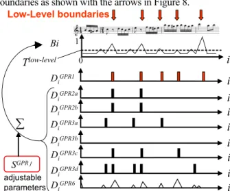
Figure 8 is the result of applying the local-level grouping rules, such as GPR1, 2a, 2b, 3a, 3d and 6¹. We calculate the degree of low-level boundary Bi as the weighted sum- mation on the local-level grouping rules results DiGPR and adjustable parameter S^{GPR j}. The threshold T^low-level decides

1The GTTM define the GPR6 for large-level grouping rules. However, we also include it for low-level grouping rules, as manual analyzing results based on GTTM by musicology experts.

if there is a low-level boundary or not. In this case, seven positions are over the threshold and five positions are applied to GPR1. Therefore, we can acquire five low-level boundaries as shown with the arrows in Figure 8.

T^low-level 0 i

1

D_i^GPR1 i D_i^GPR2a i D_i^GPR2b i D_i^GPR3a i D_i^GPR3b i Bi

D_i^GPR3c i D_i^GPR3d i D_i^GPR6 i

Low-Level boundaries

adjustable parameters

S^{GPR j}

∑

Figure 8. Detection of low-level boundaries.

5.2 Detection of high-level boundaries

The hierarchical grouping structure is constructed in the top-down method (Figure 9). First of all, consider a whole score as a group and calculate the degree of high- level boundary Di high-level boundary. Then select the strongest boundary for the next level grouping boundary as shown with the upward arrows in Figure 9. Finally iterate while the group contains low-level boundaries.

… Low-level boundaries

Calculate this way the degree of high-level boundary iteratively i

0

i i

0 0 boundary level high

Di ⁻

boundary level high

Di ⁻

boundary level high

Di ⁻

Time-span tree

adjustable parameters Grouping structure

Metrical Structure

Figure 9. Construction of hierarchical grouping structure .

6 EXPERIMENTAL RESULTS

We evaluated the performance of the music analyzer using an F-measure, which is given by the weighted harmonic mean of Precision P and Recall R,

R P

R F_measure P

+

× ×

=2 . (5) This evaluation required us to prepare correct data of a grouping structure, metrical structure, and time-span tree. We collected a hundred pieces of 8-bar length, monophonic, classical music pieces, and asked musicology experts to manually analyze them faithfully with regard to the GTTM, using the manual-edit mode of Java GUI to assist in editing the grouping structure,

(6)

metrical structure, and time-span tree. Three other experts crosschecked these manually produced results.

To evaluate the baseline performance of our system, we used the following default parameters: S^rules=0.5, T^rules=0.5, Ws,=0.5 Wr =0.5, Wl=0.5, and σ=0.05.

In the current stage, the parameters are configured by humans, because the optimal values of the parameters depend on a piece of music. When a user changes the parameters, the hierarchical structures change as a result of the new analysis.

It took us an average of about 10 minutes per piece to find the plausible tuning for the set of parameters (Table 1).

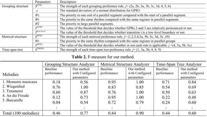
As a result of configuring the parameters, each F-measure of our analyzer outperformed the baseline (Table 2).

7 CONCLUSION

We developed a music analyzing system called ATTA, which derives the time-span tree of the GTTM. The following three points are the main results of this study.

- Proposed extended GTTM

We propose an extended GTTM for computer implementation. The difficulty with the computer implementation of GTTM has been designated, however no radical solutions have been proposed [17].

We re-formalized the rules using a numerical expression with adjustable parameters, so that it can separate the definition and ambiguity from the analyzed material.

- Implemented ATTA on computer

We implemented an actual working system to acquire the hierarchical grouping structure, metrical structure, and time-span tree of music, based on the GTTM. The ATTA automatically acquirers the time- span tree by configuring the parameters without manually analyzing by experts in musicology.

- Constructed a set of correct data

We made a set of one hundred correct data, which is the greatest database of analyzed results from the GTTM to date. We plan to exhibit this database in the near future.

- Evaluated the performance of ATTA

Our experimental results showed that, as a result of configuring the parameters, our music analyzer outperformed the baseline F-measure. The set of parameters that was tuned for a certain family of music pieces would possibly reflect the common features of the family. Thus, the idealized parameter set for a music family, if any, would expectedly analyze a new piece correctly, priort to human analysis.

We plan to develop further systems, using time-span trees and the results of the music analyzer, for other musical tasks, such as searching, harmonizing, voicing, and ad-lib to indicate the effectiveness of implementing the GTTM to provide music knowledge.

REFERENCES

[1] Lerdahl, F., and Jackendoff, R. A Generative Theory of Tonal Music. MIT Press, Cambridge, 1983.

[2] Cooper, G., and Meyer, L. B. The Rhythmic Structure of Music. The University of Chicago Press, 1960.

[3] Narmour, E. The Analysis and Cognition of Basic Melodic Structure. The University of Chicago Press, 1990.

[4] Temperley, D. The Congnition of Basic Musical Structures. MIT press, Cambridge, 2001.

[5] Hirata, K., and Matsuda, S. Interactive Music Summarization based on Generative Theory of Tonal Music. Journal of New Music Research, 32:2,

Table 2.F-measure for our method.

Grouping Structure Analyzer Metrical Structure Analyzer Time-Span Tree Analyzer Melodies

Baseline performance

Our method with Configured parameters

Our method with Configured parameters 1. Moments musicaux

2. Wiegenlied 3. Traumerei 4. An die Freude 5. Barcarolle

0.18 0.76 0.60 0.12 0.04 :

0.56 1.00 0.87 0.73 0.54 :

0.95 0.83 0.76 0.95 0.72 :

1.00 0.85 1.00 1.00 0.79 :

0.71 0.54 0.50 0.22 0.24 :

0.84 0.69 0.63 0.48 0.60 :

Total (100 melodies) 0.46 0.77 0.84 0.90 0.44 0.60

Parameters Description

S^{GPR j} The strength of each grouping preference rule. j= (2a, 2b, 3a, 3b, 3c, 3d, 4, 5, 6)

σ The standard deviation of a normal distribution for GPR5.

Ws The priority to one end of a parallel segment compared with the start of a parallel segment.

Wr The priority to the same rhythm compared with the same register in parallel segments.

Wl The priority to large parallel segments.

T^GPR4 The value of the threshold that decides whether GPRs 2 and 3 are relatively pronounced or not.

Grouping structure

T^low-level The value of the threshold that decides whether transition i is a low-level boundary or not.

S^{MPR j} The strength of each metrical preference rule. j= (1,2,3,4,5a, 5b, 5c, 5d, 5e ,10)

Wr The priority to the same rhythm compared with the same register in parallel groups.

Metrical structure

T^{MPR j} The value of the threshold that decides whether or not each rule is applicable. j =(4, 5a, 5b, 5c)

Time-span tree S^{TSRPR j} The strength of each time-span tree preference rule. j= (1, 3a, 3b, 4, 8, 9)

Table 1.Adjustable parameters.

(7)

165-177, 2003.

[6] Todd, N. A Model of Expressive Timing in Tonal Music. Musical Perception, 3:1, 33-58, 1985.

[7] Widmer, G. ''Understanding and Learning Musical Expression'', Proceedings of International Computer Music Conference, pp. 268-275, 1993.

[8] Hirata, K., and Hiraga, R. ''Ha-Hi-Hun plays Chopin’s Etude'', Working Notes of IJCAI-03 Workshop on Methods for Automatic Music Performance and their Applications in a Public Rendering Contest, pp. 72-73, 2003.

[9] Hirata, K., and Matsuda, S. ''Annotated Music for Retrieval, Reproduction, and Sharing'', Proceedings of International Computer Music Conference, pp.

584-587, 2004.

[10] Ida, K., Hirata, K., and Tojo, S. '' The Attempt of the Automatic Analysis of the Grouping Structure and Metrical Structure based on GTTM'', Proceedings of International Computer Music Conference, SIG Technical Report, 2001(42):49-54, 2001 (in Japanese).

[11] Touyou, T., Hirata, K., Tojo, S., and Satoh, K. '' Improvement of Grouping Rule Application in Implementing GTTM'', Proceedings of International Computer Music Conference, SIG Technical Report, 2002(47):121-126, 2002 (in Japanese).

[12] Nord, T. A. Toward Theoretical Verification:

Developing a Computer Model of Lerdahl and Jackendoff’s Generative Theory of Tonal Music.

Ph.D. Thesis, The University of Wisconsin, Madison, 1992.

[13] Hewlett, W. B. ed. Melodic Similarity Concepts, Procedures, and Applications, Computing in Musicology 11, The MIT press, Cambridge, 1998.

[14] Recordare LLC. MusicXML 1.0 Tutorial.

http://www. recordare.com/xml/musicxml- tutorial.pdf., 2004.

[15] W3C. XML Pointer Language (XPointer).

http://www.w3.org/TR/xptr/, 2002.

[16] W3C. XML Linking Language (XLink) Version 1.0. http://www.w3.org/TR/xlink/, 2001.

[17] Heikki, V. Lerdahl and Jackendoff Revisited.

http://www.cc.jyu.fi/~heivalko/articles/lehr_jack.htm.

Appendix 1: Grouping Structure analyzer

Step 1: Calculation of basic parameters

Six basic parameters for note transition i are calculated from MusicXML: resti (interval between current offset and next onset), ioii (inter-onset intervals), regii (pitch intervals), leni (subtraction of duration), dyni (subtraction of dynamics), and arti (subtraction of ratio between duration of performed note and proper duration of the note).

Step2: Application of GPR GPR1 (Alternative form)

⎩⎨

⎧ ≤ ≥

= ⁺

lse 0

B B

1 i-1 i 1

GPR1

e

B B

D_i and ⁱ ⁱ ,

(6)

⎟⎠

⎟⎞

⎜⎜⎝

⎛ ×

×

=

∑ ∑

= ′

=(2,2,3,3,3,3,6) ′ (2,2,3,3,3,3,6)

max

d c b a b a j

j GPR j GPR i i

d c b a b a j

j GPR j GPR i

i D S D S

Bwhere

. GPR2a (Slur/Rest)

⎩⎨

⎧ < >

= ⁻ ⁺

lse e

rest rest and rest rest

Di^GPR2a ⁱ ⁱ ⁱ ⁱ

0

1 ₁ ₁

(7) GPR2b (Attack-Point)

⎩⎨

⎧ < >

= ⁻ ⁺

lse e

ioi oi i and ioi oi i

D_i^GPR2b ⁱ ⁱ ⁱ ⁱ

0

1 1 1

(8) GPR3a (Register)

⎩⎨

⎧ < >

= ⁻ ⁺

lse e

regi regi and regi regi

Di^GPR3a ⁱ ⁱ ⁱ ⁱ

0

1 ₁ ₁

(9) GPR3b (Dynamics)

⎩⎨

⎧ = ≠ =

= ⁻ ⁺

lse e

dyn and 0 dyn and dyn

Di^GPR3b ⁱ ⁱ ⁱ

0

0 0

1 ₁ ₁

(10) GPR3c (Articulation)

⎩⎨

⎧ = ≠ =

= ⁻ ⁺

lse e

and arti and arti

D_i artiⁱ ⁱ ⁱ

0

0 0

0

1 ₁ ₁

GPR3c (11)

GPR3d (Length)

⎩⎨

⎧ = ≠ =

= ⁻ ⁺

lse 0

0 len and 0 len and 0 len

1 ₁ ₁

GPR3d

D_i e ⁱ ⁱ ⁱ (12)

GPR4 (Intensification)

( )

⎩⎨

⎧ >

= 0 lse

P , P , P , P , P max 1

4 arti

i dyn i regist i ioi i rest i GPR4

e D T

GPR i

(13)

arti arti P , lse 0

0 regi regi P regi

, dyn dyn P ,

P , rest rest P

1 1 i arti i 1

1 1

1 regist i

i

1 1 i dyn i 1

1 i ioi i 1

1 i rest i

∑ ∑

∑

+

−

= +

−

= +

−

=

+

−

= +

−

= +

−

=

⎪ =

⎩

⎪⎨

⎧

⎟⎟⎠

⎜⎜ ⎞

⎝

⎛ >

=

i i j

j i

i j

j i

i j

j

i i

j j

i i

j j

i i

j j

e ioi ioi

GPR5 (Symmetry) where

.

⎪⎭

⎪⎬

⎫

⎪⎩

⎪⎨

⎧ ⎟

⎠

⎜ ⎞

⎝

⎛ ∑ − ∑

−

= = =

2 2

GPR5 exp ^end 2 2σ

start

j j

i start

j j

i ioi ioi

D , (14)

start : start transiton of a group.

where

end : end transition of a group.

GPR6 (Parallelism)

( )

∑ ∑

⎪⎪

⎪

⎩

⎪⎪

⎪

⎨

⎧

=

× +

−

×

=

×

=

−

×

=

j r

j i j i end s

r j i start s

r j i

j i end s

r j i

j i start s

r j i iGPR6

m

m W G W G

m W G

D

s 0

t 1

e b 1

, (15)

where

division : duration of a quarter note.

r : length of parallel segments based on the division of a quarter note.

Wl r r r j- q r i- q

r r j- q r i- l q r W r r j- q r i- q

r r j- q r i- end q

j i

Wl r r j q i q

r j q i l q r W r j q i q

r j q i start q

j i

r z W

r y y W

G z

r z W

r y y W

G z

+ +

×

× +

×

−

×

=

×

× +

×

−

×

=

1 1

) 1 (

( ^Gausian^integer)

division ioi

q ⁱ

k k

i []:

1 ⎥⎦

⎢ ⎤

⎣

=⎡∑

=

⎪⎪

⎩

⎪⎪

⎨

⎧

≠

=

≠

=

+ +

lse e s

q q and q q and q q and q q t

q q and q q and q q and q q e

q q and q q and q q and q q m

1 j j 1 i i 1 - j j 1 - i i

j i

b

∑⎩⎨⎧ ≤ ≤ +

=

j

i j j i ir

q 0 else

r q q and q q

x 1