On Necessary Conditions for Dependence Parameters of Minimum and Maximum Value Distributions Based on n-Variate FGM Copula

586 IEICE TRANS. FUNDAMENTALS, VOL.E102–A, NO.3 MARCH 2019

LETTER

On Necessary Conditions for Dependence Parameters of Minimum and Maximum Value Distributions Based on n-Variate FGM Copula

Shuhei OTA^†,Student Member andMitsuhiro KIMURA^††a),Senior Member

SUMMARY This paper deals with the minimum and maximum value distributions based on then-variate FGM copula with one dependence pa- rameter. The ranges of dependence parameters are theoretically determined so that the probability density function always takes a non-negative value.

However, the closed-form conditions of the ranges for the dependence pa- rameters have not been known in the literature. In this paper, we newly provide the necessary conditions of the ranges of the dependence parame- ters for the minimum and maximum value distributions which are derived from FGM copula, and show the asymptotic properties of the ranges.

key words: minimum value distribution, maximum value distribution, FGM copula, dependence parameter, asymptotic properties

1. Introduction

Dependence modeling with copulas is one of the challenging research topics of statistical modeling in the last decade. An n-variate copula is a multivariate distribution function hav- ingnuniform marginal distributions on the interval [0,1] (cf., [1]and[2]). Copulas provide powerful tools in the multi- variate statistical analysis because one can construct various dependence models by replacing the uniform marginal dis- tributions with other marginal distributions. In particular, the Farlie-Gumbel-Morgenstern (FGM, for short) copula is useful as an alternative to a multivariate normal distribution because it has a simple form and it can express mutual depen- dencies among two or more variables. Therefore, the FGM copula has been applied to the statistical modeling in differ- ent research fields such as reliability engineering, finance, economics, and so on (e.g.,[3]and[4]). For more details about the bivariate FGM copula, see[5]and[6]. In addition, [7]and[8]well explained then-variate FGM copula.

One unresolved problem of the FGM copula is that re- strictions of its parameters have not been found as closed forms. For this reason, for example, it has been difficult to estimate the dependence parameters of the FGM copula so far. Then-variate FGM copula proposed by[7]has to- tally 2ⁿ−n−1 dependence parameters which describe the dependencies among the variables (N.B.,_n

2

parameters of them are for the dependencies between any two variables, _n

3

parameters of them are for among any three variables, and so on). Note that the parameters should be determined so that its joint density function is always non-negative[7].

Manuscript received November 7, 2018.

†The author is with Graduate School of Science & Engineering, Hosei University, Koganei-shi, 184-8584 Japan.

††The author is with Faculty of Science & Engineering, Hosei University, Koganei-shi, 184-8584 Japan.

a) E-mail: [email protected]

DOI: 10.1587/transfun.E102.A.586

In general, a lot of papers have referred to this restriction (e.g.,[2],[9], and[10]). However, there are few studies that explicitly derive the exact ranges of the parameters forn≥4 in particular because of its complexity.

Under such a situation, as a first step, we focus on the minimum and maximum value distributions which are con- structed by the n-variate FGM copula in this paper. The former distribution can describe the lifetime (first failure occurrence time) of a series system withndependent com- ponents, and the latter one does that of a dependent parallel system. In addition, in order to reduce the complexity in- volved in the n-variate FGM copula, we assume that all dependence parameters are represented by just one parame- ter. As a result, the necessary conditions for the dependence parameter of minimum and maximum distributions are ex- plicitly provided.

In the following section, we explain the fundamental feature of the n-variate FGM copula, and Sect. 3 presents the necessary conditions of the dependence parameters for any givenn. The derivation methods of them are presented in Sect. 4. Some discussion on the sufficient conditions and remaining issues on this topic is briefly referred in Sect. 5.

2. Definition

SupposeU = (U₁,U₂, . . . ,U_n)be a random vector that fol- lows an FGM copula withnuniform marginal distributions on the interval [0,1]. LetCbe the joint distribution func- tion of the n-variate FGM copula and letF be the sub- sets which consist of all combinations of at least two ele- ments of an index set{1,2, . . . ,n}. For example, ifn =3, F ={{1,2},{1,3},{2,3},{1,2,3}}. Denote thatθ is a vec- tor representation of the dependence parameter set of the FGM copula. Then, according to[7], the joint distribution function ofUcan be written by

C(u₁,u₂, . . . ,u_n;θ)

=Pr[U₁ ≤u₁,U₂≤u₂, . . . ,U_n ≤u_n]

=

n

Y

i=1

u_i* . ,

1+X

S∈F

α_SY

j∈S

(1−u_j)+ / -

, (1)

whereα_S’s are the elements of the dependence parameters (i.e., (α_S ∈ θ)). Moreover, its joint density function is expressed by the following form:

c(u₁,u₂, . . . ,un;θ)

Copyright © 2019 The Institute of Electronics, Information and Communication Engineers

LETTER

587

= ∂ⁿ

∂u₁∂u₂· · ·∂u_nC(u₁,u₂, . . . ,u_n;θ)

=1+ X

S∈F

α_SY

j∈S

(1−2uj). (2)

Note thatθis the parameter set such that the joint den- sity function is non-negative for everyu_i ∈ [0,1]. Thus it is easy to see thatα_S’s must satisfy the following limitation (cf.,[1]).

1+ X

S∈F

α_SY

j∈S

(1−2u_j)≥0, (3)

for∀(u₁,u₂, . . . ,u_n)∈[0,1]ⁿ. Consequently, for the simplest case,n=2, the parameter set becomesθ ={α{1,2}}and we have the well-known range−1≤α{1,2}≤1 from Eq. (3).

In the case ofn=3, the parametersθ={α{1,2},α{1,3}, α{2,3},α{1,2,3}}are required to hold the following conditions (cf.,[7]and[12]).

1+α{1,2}+α{1,3}+α{2,3}≥ |α{1,2,3}| 1+α{1,2}−α{1,3}−α{2,3}≥ |α{1,2,3}| 1−α{1,2}+α{1,3}−α{2,3}≥ |α{1,2,3}| 1−α{1,2}−α{1,3}+α{2,3}≥ |α{1,2,3}|















. (4)

The ranges of these dependence parameters must be deter- mined so as to satisfy Eq. (4). However, it is not so easy to find them. Johnson and Kotz[7]added an additional con- dition such that∀α_S =0 for|S| <nin order to loosen the restriction (N.B.,|S|means the size of the setS). Then the exact range ofα{1,2,...,n}can be obtained as

−1≤α{1,2,...,n}≤1. (5)

As a result, we can see that it is very hard to derive the exact ranges of the dependence parameters unless some certain conditions are made. Therefore in this paper, as we mentioned in Sect. 1, we try to obtain the ranges of the de- pendence parameters for the minimum and maximum value distributions based on then-variate FGM copula when all of the dependence parameters are identical toθ. That is, we assume thatθ≡α_Sfor allSin Eq. (1).

3. Main Results

We first show the minimum and maximum distribution func- tions derived from one-parameter n-variate FGM copula.

LetU_1:nandU_n:nbe the minimum and maximum values of U, respectively. C_1:n(u;θ_1:n) andC_n:n(u;θ_n:n) denote the cumulative distribution functions (CDF) ofU_1:n andU_n:n, respectively. According to [11]and [12], C_1:n(u;θ_1:n) is obtained as

C_1:n(u;θ_1:n)=Pr[min(U₁,U₂, . . . ,U_n)≤u]

=1−(1−u)ⁿ* ,

1+θ_1:n

n

X

k=2

n k

! (−u)^k+

-

. (6)

AlsoC_n:n(u;θ_n:n)is given by

C_n:n(u;θ_n:n)=Pr[max(U₁,U₂, . . . ,U_n)≤u]

=uⁿ* ,

1+θ_n:n Xn

k=2

n k

!

(1−u)^k+ -

. (7)

Note that we rewrite θ to θ_1:n andθ_n:n in the above equations respectively in order to distinguish these two pa- rameters.

The following theorems present the necessary condi- tions for the ranges of θ_1:n and θ_n:n in Eqs. (6) and (7), respectively. In addition, these theorems yield corollaries about their asymptotic properties.

Theorem 3.1: The range ofθ_1:n is given by the following inequality.

− 1

n−1 ≤θ_1:n≤ 1

2−2(1−u^∗_n)ⁿ−(1+n)u^∗_n, (8) where

u^∗_n=1− 1+n 2n

!_n−¹₁

. (9)

Corollary 3.1: Asn→ ∞, the range ofθ_1:nis obtained as 0≤θ_1:n ≤ 1

1−log2'3.259. (10)

Theorem 3.2: The range ofθ_n:nis given by the following inequality.

− 1

2ⁿ−1−n ≤θ_n:n ≤ 1

(1−v_n^∗){1+n−2(2−v_n^∗)ⁿ⁻¹}, (11) wherev_n^∗is uniquely defined by the solution of the following equation.

n(2−v_n^∗)ⁿ⁻¹−(n−1)(2−v_n^∗)ⁿ⁻²−1+n

2 =0, (12) for 0≤v_n^∗≤1.

Remark 3.1: The asymptotic property ofv_n^∗is as follows.

n→∞lim v_n^∗ =1. (13)

This remark offers some support to the next conjecture.

Conjecture 3.1: Asn→ ∞, the following equation holds.

n→∞lim

1

(1−v_n^∗){1+n−2(2−v_n^∗)ⁿ⁻¹} =0. (14) This conjecture is derived byRemark 3.1and the assump- tion that 1+n−2(2−v_n^∗)ⁿ⁻¹ diverges to positive infinity more quickly than 1−v_n^∗converges to 0. Then we have the following corollary.

Corollary 3.2: Asn→ ∞, the range ofθ_n:nis convergent to 0.

588 IEICE TRANS. FUNDAMENTALS, VOL.E102–A, NO.3 MARCH 2019

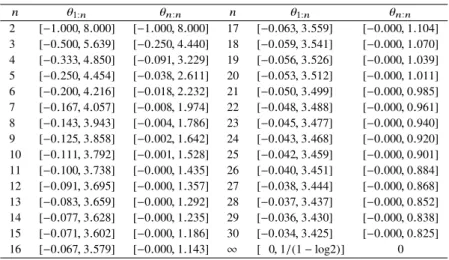
Table 1 Numerical results of the ranges ofθ_1:nandθn:n.

n θ_1:n θn:n n θ_1:n θn:n

2 [−1.000,8.000] [−1.000,8.000] 17 [−0.063,3.559] [−0.000,1.104]

3 [−0.500,5.639] [−0.250,4.440] 18 [−0.059,3.541] [−0.000,1.070]

4 [−0.333,4.850] [−0.091,3.229] 19 [−0.056,3.526] [−0.000,1.039]

5 [−0.250,4.454] [−0.038,2.611] 20 [−0.053,3.512] [−0.000,1.011]

6 [−0.200,4.216] [−0.018,2.232] 21 [−0.050,3.499] [−0.000,0.985]

7 [−0.167,4.057] [−0.008,1.974] 22 [−0.048,3.488] [−0.000,0.961]

8 [−0.143,3.943] [−0.004,1.786] 23 [−0.045,3.477] [−0.000,0.940]

9 [−0.125,3.858] [−0.002,1.642] 24 [−0.043,3.468] [−0.000,0.920]

10 [−0.111,3.792] [−0.001,1.528] 25 [−0.042,3.459] [−0.000,0.901]

11 [−0.100,3.738] [−0.000,1.435] 26 [−0.040,3.451] [−0.000,0.884]

12 [−0.091,3.695] [−0.000,1.357] 27 [−0.038,3.444] [−0.000,0.868]

13 [−0.083,3.659] [−0.000,1.292] 28 [−0.037,3.437] [−0.000,0.852]

14 [−0.077,3.628] [−0.000,1.235] 29 [−0.036,3.430] [−0.000,0.838]

15 [−0.071,3.602] [−0.000,1.186] 30 [−0.034,3.425] [−0.000,0.825]

16 [−0.067,3.579] [−0.000,1.143] ∞ [ 0,1/(1−log2)] 0

In summary, the above results guarantee that the ranges ofθ_1:n andθ_n:n depend on onlyn, and the ranges become narrower as n increases. For example, Table 1 shows the numerical results of the ranges of θ_1:n and θ_n:n for n = 2,3, . . . ,30,and∞. Note that every value is calculated by Eqs. (8) and (11), and rounded to the nearest thousandth.

This table implies that the ranges of the negative values of θ_1:nandθ_n:nare narrower than those of the positive values, respectively. In addition, we can find that the range ofθ_n:n is narrower than that ofθ_1:n.

4. Proofs

Proof of Theorem 3.1:We need to derive the closed form of the limitationθ_1:n ∈ {θ| ^d

duC_1:n(u;θ)≥0,0≤u≤1}. First we define the probability density function (PDF) ofU_1:nby the followingc_1:n(u;θ_1:n).

c_1:n(u;θ_1:n)= d

duC_1:n(u;θ_1:n)

=n(1−u)ⁿ⁻¹1+θ_1:n(−2+2(1−u)ⁿ+(1+n)u) . (15) Here,θ_1:nhas the following relationship.

θ_1:n∈ {θ|c_1:n(u;θ)≥0,0≤u≤1}

⇔θ_1:n ∈ {θ| min

0≤u≤1[c_1:n(u;θ)]≥0}. (16) That is, the problem is equivalent to findingθ_1:n such that the minimum value ofc_1:n(u;θ_1:n) is non-negative. Since n(1−u)ⁿ⁻¹ ≥0 for 0≤u≤1 andn≥2, we have

θ_1:n∈ {θ| min

0≤u≤1[ ˜c_1:n(u;θ)]≥0}, (17) where

˜

c_1:n(u;θ_1:n)= 1

n(1−u)ⁿ⁻¹c_1:n(u;θ_1:n). (18) Hence, we can verify theTheorem 3.1by solving the mini- mization problem of Eq. (17). In order to solve this problem,

we define the first and second derivatives with respect tou of ˜c_1:n(u;θ_1:n)as follows.

˜

c_1:n⁰ (u;θ_1:n)^def= d

duc˜_1:n(u;θ_1:n)

=θ_1:n(−2n(1−u)ⁿ⁻¹+1+n), (19)

˜

c_1:n⁰⁰ (u;θ_1:n)^def= d²

du²c˜_1:n(u;θ_1:n)

=θ_1:n(n−1)n(1−u)ⁿ⁻². (20) Letu^∗_n be an critical point of ˜c_1:n(i.e., ˜c_1:n⁰ (u^∗_n;θ_1:n) =0).

Then,u^∗_nuniquely exists on the interval [0,1], and it is easy to see thatu^∗_n =1−_1+n

2n

_n−¹₁

Consider θ_1:n ≥ 0. In this case, for 0. ≤ u ≤ 1,

˜

c_1:n(u;θ_1:n)is a convex function because ˜c_1:n⁰⁰ (u;θ_1:n) ≥0.

Thus, ˜c_1:n(u^∗_n;θ_1:n)is the absolute minimum value. Hence, we haveθ_1:n ∈ {θ|c˜_1:n(u^∗_n;θ) ≥0}. This yields

θ_1:n ≤ 1

2−2(1−u^∗_n)ⁿ−(1+n)u^∗_n, (21) where 1/(2−2(1−u^∗_n)ⁿ−(1+n)u^∗_n)gives the upper bound ofθ_1:n.

Considerθ_1:n < 0. In this case, ˜c_1:n(u;θ_1:n)is a con- cave function that takes the minimum value if and only if u = 1. Thus, we have θ_1:n ∈ {θ | c˜_1:n(1;θ) ≥ 0}. This implies

− 1

n−1 ≤θ_1:n, (22)

where−1/(n−1)gives the lower bound ofθ_1:n. Hence, the proof is complete.

Proof of Corollary 3.1: ByTheorem 3.1, the upper bound ofθ_1:nis given by 1/(2−2(1−u^∗_n)ⁿ−(1+n)u^∗_n). Thus as n→ ∞, the upper bound ofθ_1:ncan be written by

n→∞lim

1

2−2(¹⁺_2nⁿ)ⁿ⁻ⁿ¹ −(1+n)(1−¹⁺_2nⁿ)ⁿ⁻¹¹

. (23)

Note thatu^∗_nis replaced by Eq. (9). By considering its Taylor

LETTER

589

series, Eq. (23) equals to

n→∞lim

1

2−(1+O(_n¹))−(log 2+O(_n¹)) = 1 1−log 2,

(24) whereO(·)denotes Landau’s symbol.

Moreover, for the lower bound, we have

n→∞lim− 1

n−1 =0. (25)

Hence, the proof is complete.

We would like to omit the proofs ofTheorem 3.2and Corollary 3.2because they can be shown in the same way as those ofTheorem 3.1andCorollary 3.1.

5. Discussion and Concluding Remarks

The results in the previous section have been obtained from the necessary condition such that Eq. (15) always takes non- negative value for any u ∈ [0,1] and n in the case of the minimum value distribution (and the maximum one as well).

Therefore the ranges obtained by Eqs. (8) and (11) are both lack of sufficiency. In order to show this fact, let us go back to the FGM copula presented in Eq. (1) with n = 3. By setting all the parametersα{1,2},α{1,3},α{2,3}, andα{1,2,3}be identical toθin Eq. (4), we can calculate the possible range ofθas

−1

4 ≤θ≤ 1

2. (26)

On the other hand, from Table 1, we recall

−1

2 ≤θ_1:3≤5.639, (27)

−1

4 ≤θ_3:3≤4.440, (28)

for the two kinds of dependence parameters, respectively. It should be noted that the minimum and maximum value dis- tributions which have been dealt with in this paper both exist only if the n-variate FGM copula is theoretically valid. In other words, for example, if we estimate that the value of ˆθ_1:3is 2.0 from a certain data analysis concerning

the minimum value distribution, this value surely satisfies Eqs. (8) and (27) but it does not satisfy the limitation de- noted by Eq. (3) with the identical dependence parameters.

Therefore in this case, we must discard the estimation result θˆ_1:3 = 2.0, and need to find the estimated value from the range−¹₄ ≤θ≤ ¹₂ in Eq. (26) instead of Eq. (27).

In conclusion, we have revealed the necessary condi- tions for the dependence parametersθ_1:nandθ_n:nfor general nand their asymptotic properties onn → ∞in this paper.

However, providing their sufficient conditions and the ex- act ranges of the parameters has been still remaining for the future work.

References

[1] P. Jaworski, F. Durante, W. Härdle, and T. Rychlik, eds., Copula Theory and Its Applications, Springer-Verlag, Berlin, 2010.

[2] R.B. Nelsen, An Introduction to Copulas, second ed., Springer- Verlag, Portland, 2010.

[3] S. Eryilmaz and F. Tank, “On reliability analysis of a two-dependent- unit series system with a standby unit,” Appl. Math. Comput., vol.218, no.15, pp.7792–7797, April 2012.

[4] H. Cossette, M.P. Cote, E. Marceau, and K. Moutanabbir, “Multi- variate distribution defined with Farlie-Gumbel-Morgenstern copula and mixed Erlang marginals: Aggregation and capital allocation,”

Insurance Math. Econom, vol.52, no.3, pp.560–572, May 2013.

[5] D.J. Farlie, “The performance of some correlation coefficients for a general bivariate distribution,” Biometrika, vol.47, no.3-4, pp.307–

323, Dec. 1960.

[6] E.J. Gumbel, “Bivariate exponential distributions,” J. Am. Stat. As- soc., vol.55, no.292, pp.698–707, Dec. 1960.

[7] N.L. Johnson and S. Kotz, “On some generalized Farlie-Gumbel- Morgenstern distributions,” Commun. Stat., vol.4, no.5, pp.415–427, Oct. 1975.

[8] D.D. Mari and S. Kotz, Correlation and Dependence, Imperial Col- lege Press, London, 2001.

[9] S. Cambanis, “Some properties and generalizations of multivariate Eyraud-Gumbel-Morgenstern distributions,” J. Multivariate Annal., vol.7, no.4, pp.551–559, Dec. 1977.

[10] E. Hashorva, “Asymptotic results for FGM random sequences,”

Statist. Probab. Lett., vol.54, no.4, pp.417–425, Oct. 2001.

[11] J. Navarro, J.M. Ruiz, and C.J. Sandoval, “Properties of coherent systems with dependent components,” Commun. Stat., vol.36, no.1, pp.175–191, Feb. 2007.

[12] M. Kimura, S. Ota, and S. Abe, “Some reliability properties ofn- component parallel/series systems with interdependent failures,” in Reliability Modeling with Computer and Maintenance Applications, S. Nakamura, C.H. Qian, and T. Nakagawa, eds., pp.155–173, World Scientific, Singapore, 2017.