An Augmented A/P/C Cohort Model : Applications
Part I : Changes in Household Demand for Wine in Japan
Part II : Estimating Impacts of the O-157 and BSE Incidents on Japanese
At-Home Beef Consumption Using an Augmented Cohort Model
Hiroshi Mori*, Hayden Stewart**, and Yoshiharu Saegusa***
Part I : Changes in Household Demand for Wine in Japan : Economic and
Demographic Aspects
Hiroshi Mori, Hayden Stewart, and Yoshiharu Saegusa
AbstractAlcohol consumption (per adult) in Japan increased by 30% between 1980 and the mid-1990s. It then declined by 10% between then and 2010. The consumption of wine, a relative new-comer to Japan’s alcohol market, also grew sharply up to a point in the 1990s before falling off. Still, consumption quadrupled over the period as a whole. This study analyzes the effects of prices, income, aging, and generational change on at-home wine consumption from 1979 to 2011. Japan experienced rapid economic growth during the past handful of decades. This, in turn, led to changes in food consumption patterns with people born around the same point in history exhibiting more similar food choices than people born farther apart in time. We find that Japanese born between 1955 and 1979 exhibit the greatest demand for wine. How-ever, “pure” period effects have had a greater impact on wine consumption than demo-graphic changes. Also, when per−adult wine consumption was regressed against real prices and real household expenditures (a proxy for income), we obtained estimates of the price elasticity as large as −3.3. However, when accounting for demographic determinants of de-mand, we obtained an average price elasticity of −0.8 and negligible income elasticity.
JEL Classification : D12, C4, Q13
Keywords : Wine, Augmented Cohort Analysis, Price Elasticity, Pure Period Effects
* Professor Emeritus, Senshu University.
** Economist, Economic Research Service, U.S. Department of Agriculture. ***Professor of Statistics (retired), Tokyo Metropolitan University.
1. Introduction
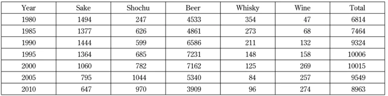
Total alcoholic beverage consumption in Japan increased sharply from 6,814 thousand kiloliters (tkl) in 1980 to 9,324 tkl in 1990, more slowly to 10,015 tkl in 2000, and then gradually declined to 8,963 tkl in 2010 (Table 1)1
. Japanese traditionally drank “sake”, brewed mainly from rice with 12%−15% alcoholic content, along with beer and “shochu”, spirits brewed from sweet potato, barley and/or rice with 25%−35% alcoholic content. Whisky and particularly wine are relatively new drinks in Japan.
Forty years ago, sake accounted for nearly half of household expenditures spent on alcoholic bev-erages, followed by beer (34%) and whisky (about 10%). Sake expenditures have declined consis-tently since 1970. Household consumption of whisky has followed suit since 1980. However, beer, shochu, and wine have followed a different trajectory, with wine and shochu showing strong, consis-tent growth in household expenditures (Tables 2 and 3).
Domestically produced wine accounted for a little over 30% of Japan’s wine market in the 2000s, steadily declining from 70% in the early 1980s (e.g., Japan Winery Association, 2012). Imported wine has conversely risen to account for nearly 70% of total consumption. Major suppliers include France (40%−50% market share of Japan’s imports in the late 2000s), Italy (20%), Chile (12%−15%), Spain (7% −10%), the U.S. (7%−9%), and Australia (6%−7%). Domestically produced wine includes wine brewed from domestically produced grapes blended with wine imported in bulk. It is estimated that “75 per-cent of domestically produced volumes” are produced with imported ingredients (USDA, GAIN Re-port, 2/23/2011, pp. 5−6). International interest in Japan’s wine market has recently motivated re-search on the determinants of consumption (Arahata, 2004 ; Rod and Beal, 2012 among the few). Rod and Beal (2012), for one, note that Japan’s wine market is subject to “fads and fashions” (p. 10). For example, in the late 1990s, consumption grew rapidly due to reports about the potential health benefits of drinking red wine. However, much work remains to be done. Still needed are accurate price and income elasticities as well as a better understanding of how consumption varies by some key demographic characteristics.
Changes in prices and income do not appear to explain all of the changes in the composition of Japan’s market for alcohols. Japan’s economy expanded very rapidly during the 1980s. The eco-nomic bubble then burst in the early 1990s. However, even as household income has changed rela-tively little since that time, trends in alcohol consumption have not stabilized. Shown in Table 2 are price trends over these same years. The figures in the parentheses of each cell in Table 2 denote
Table 1. Consumption of Alcoholic Beverages in Japan, 1980 to 2010 (1000 kl)
Year Sake Shochu Beer Whisky Wine Total
1980 1494 247 4533 354 47 6814 1985 1377 626 4861 273 68 7464 1990 1444 599 6586 211 132 9324 1995 1364 685 7231 148 158 10006 2000 1060 782 7162 125 269 10015 2005 795 1044 5340 84 257 9549 2010 647 970 3909 96 274 8963
Note : Quantities in terms of taxed volume.
the consumer price index (CPI) for each individual product divided by the aggregate CPI with 2005 =100. Real consumer prices for sake have stayed almost constant for the past 40 years and yet per− household consumption of sake has consistently shrunk. By contrast, real prices for shochu seem to have risen slightly, partly reflecting higher levels of quality, perhaps, but household consumption has quadrupled. Real consumer prices for wine have declined gradually over the past 30 years con-current with steadily increasing consumption.
The demand for alcohols as well as many types of food varies among Japanese according to some key demographic characteristics of the individual. Japan is an aging society that has also experi-enced rapid economic growth and become much more internationalized over the past handful of decades. This, in turn, has led to changes in food consumption patterns with people born around the same point in history exhibiting more similar food choices than people born farther apart in time. Mori, Clason, and Lillywhite (2006), for example, investigate trends in Japanese fresh fruit consumption. Increasingly younger generations were found to consume smaller quantities of fresh apples and fresh mandarin oranges than members of older generations consume.2
Mori and Saegusa (2010) similarly found that younger generations were inclined to consume less fish.3
Individuals who grew up amidst post-World War II economic prosperity are likely accustomed to a more diverse diet than are members of older generations who came of age consuming these traditional foods. Both studies use an A/P/C model that decomposes consumption into the effects of an individual’s age, “pure” period (time) effects, and his or her birth years (cohort). Pure time effects are the trend in
Table 2. Household Purchases (liters/year) and Real Prices of Alcoholic Beverages, 1970-2010
Year Sake Shochu Whisky Beer Wine
1970 22.08 (119) 2.13 (88) 1.84 (227) 29.57 (128) 0.44 (NA) 1980 18.31 (98) 2.63 (75) 3.19 (134) 46.76 (95) 0.55 (137) 1985 15.22 (100) 5.95 (80) 2.44 (154) 42.45 (111) 0.64 (143) 1990 13.47 (99) 4.90 (83) 1.88 (145) 55.39 (106) 0.86 (135) 1995 13.25 (104) 6.12 (88) 1.50 (135) 58.93 (103) 1.27 (124) 2000 10.83 (103) 7.01 (99) 1.16 (102) 60.16 (102) 2.40 (103) 2005 9.37 (100) 10.38 (100) 0.88 (100) 52.80 (100) 2.17 (100) 2010 7.91 (91) 10.70 (104) 0.88 (95) 54.14 (97) 2.17 (96)
Notes : Figures in parentheses denote individual CPI deflated by the aggregate CPI (base year=2005). Sources : FIES, various years.
Table 3. Household Expenditures Shares on Alcoholic Beverages (Percentages), 1970 to 2010
Year Total Sake Shochu Beer Whisky Wine
1970 100 48.7 2.8 34.0 9.6 1.0 1980 100 34.0 3.1 42.3 16.7 1.6 1985 100 28.2 7.8 46.2 12.6 1.7 1990 100 22.2 6.0 55.6 10.7 2.4 1995 100 22.2 7.1 57.9 7.2 2.5 2000 100 19.0 9.0 58.5 4.4 5.8 2005 100 16.8 15.2 52.3 2.8 5.6 2010 100 14.6 16.9 53.4 2.9 5.8
consumption controlling for other variables in the model and, in the case of trends in alcohol con-sumption, may represent the net effects of health information like reports in the 1990s that drinking red wine is healthful, marketing efforts by companies like supermarkets that allocated increased sales space to wine, and other fads and fashions on top of the economic variables of price and in-come.
Two previous studies have examined the demand for alcohol in Japan allowing for the possibility that different birth cohorts exhibit different tastes and preferences. Tanaka et al. (2004) investigated sake and beer consumption using an A/P/C model. Middle-aged Japanese (i.e., those above their mid−40s) drank more than twice as much sake as those in their 20s and 30s in the survey period, 1980−2000. Sake consumption was lower among younger birth cohorts who grew up after the high economic growth of Japan’s economy, which started in the early 1960s. Tanaka et al. (2004a) sur-mised that those in their 50s and 60s in 2010 to 2020, for example, would not drink as much sake as their counterparts did some 20−30 years ago, because they belong to newer generations who exhibit negative cohort effects in sake consumption. Providing some validation of their estimates, Tanaka et al.’s (2004) predictions of household sake consumption in 2010 coincided with actual consumption reported in the government’s Family Income and Expenditure Survey (FIES ) of 2010. Okamoto (2003) used an A/P/C model to identify cohort effects in household wine and whisky consumption. He did not, however, try to incorporate price and income effects in his modeling.
Drastic changes in the consumption structure of alcoholic beverages in the past 30−40 years in Japanese households need to be analyzed not only from the economic perspectives of price and in-come but also from the demographic perspectives of age and generations. As stated before, wine re-mains a relatively new and quickly growing product in Japan. We will investigate in this paper changes in households’ at−home wine consumption using both economic and demographic frame-works. That is, we ask which birth cohorts most prefer wine. We also estimate pure time effects and calculate income and price elasticities.
1
Alcoholic beverage consumption is measured as the taxed volume.
2
Those in their 30s are estimated to eat (approximately) 2.0kg of apples (per year ; per person) and 3.0kg of mandarin oranges, as compared to 8.0kg and 12.0kg, respectively by those in their 60s in 2000, for example (Mori et al., pp.208 −9).
3
Those in their 30s are estimated to consume 9.5kg of fresh fish (per year ; per person), as compared to 20.0kg by those in their 60s in 2004, for example (Mori and Saegusa, p.48).
2. Data
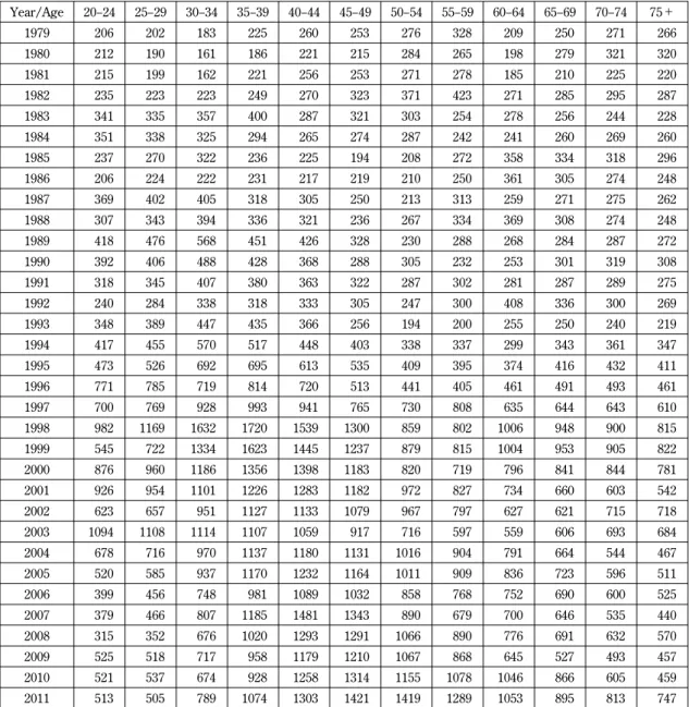
Table 4 illustrates household purchases (=consumption) of wine and shochu classified by HH age groups in 1995, the midpoint of the survey period, 1979 to 2011. The number in the second col-umn denotes the average number of persons contained in each HH age group.
The figures in the third column denote annual purchases of wine in milliliters (cc) by HH age groups. It should be noted that these figures represent household consumption, not the consump-tion of individual household members.
In order to derive estimates of per capita consumption from FIES data, researchers at the Jap-anese government research institute, PRIMAFF, among other institutions, commonly divide house-hold consumption for each age group by the size of househouse-holds in that group (e.g., PRIMAFF, 2010). Suppose, as shown below with hypothetical numbers, that households headed by individuals aged 30, 45, and 55 years consumed 20, 40, and 20 units of a food or beverage and contained 3, 4, and 3 members, respectively :
HQ30(3)=20 (1)
HQ45(4)=40 (2)
HQ55(3)=20 (3)
where HQidenotes household consumption for HH i years of age and the figures in parentheses
denote the number of persons contained in the specific household. Simple division provides per cap-ita consumption by age as follows :
Q30=20/3=6.7 (4)
Q45=40/4=10.0 (5)
Q55=20/3=6.7 (6)
where Qidenotes average per capita consumption by individuals of i years of age.
However, the above approach ignores the fact that one of the three family members of the house-hold where HH is 30 years of age is likely an infant who does not eat as much foods as his/her par-ents and never drinks alcoholic beverages at all. In the case of the household where HH is 55 years of age, one of the three members is likely a grown-up adult in their 20s, who may normally eat or drink more than his/her parents. Therefore, dividing household consumption by 3, in equation (4) might lead to a substantial underestimation of per capita individual consumption of those in their 30 s, whereas doing so in equation (6) for a household head aged 55 may likely overestimate consump-tion for this age group.
Table 4. At-home Wine Consumption by Age Groups of Household Head, 1995
Household Head Age Number of persons in Household Wine (cc) Shochu (cc)
A somewhat more accurate way to derive individual consumption estimates from household-level data, based on equivalence scales and using information on the age distribution of Japanese house-holds covered by the FIES , would be to broadly re-write equations (1) to (3) as below4
:
2Q30+1Q0=20 (7)
2Q45+1Q17=40 (8)
2Q55+1Q25=20. (9)
In reference to sporadic nutrition surveys, whenever available and by common sense, it may be safe to further assume Q0=0, Q25=Q30, and Q17=1.2*Q25for some chosen food such as pork. Then it
follows that
Table 5. Estimated per capita Wine Consumption at Home by Age, 1979-2011 (cc/Year)
Year/Age 20−24 25−29 30−34 35−39 40−44 45−49 50−54 55−59 60−64 65−69 70−74 75+ 1979 206 202 183 225 260 253 276 328 209 250 271 266 1980 212 190 161 186 221 215 284 265 198 279 321 320 1981 215 199 162 221 256 253 271 278 185 210 225 220 1982 235 223 223 249 270 323 371 423 271 285 295 287 1983 341 335 357 400 287 321 303 254 278 256 244 228 1984 351 338 325 294 265 274 287 242 241 260 269 260 1985 237 270 322 236 225 194 208 272 358 334 318 296 1986 206 224 222 231 217 219 210 250 361 305 274 248 1987 369 402 405 318 305 250 213 313 259 271 275 262 1988 307 343 394 336 321 236 267 334 369 308 274 248 1989 418 476 568 451 426 328 230 288 268 284 287 272 1990 392 406 488 428 368 288 305 232 253 301 319 308 1991 318 345 407 380 363 322 287 302 281 287 289 275 1992 240 284 338 318 333 305 247 300 408 336 300 269 1993 348 389 447 435 366 256 194 200 255 250 240 219 1994 417 455 570 517 448 403 338 337 299 343 361 347 1995 473 526 692 695 613 535 409 395 374 416 432 411 1996 771 785 719 814 720 513 441 405 461 491 493 461 1997 700 769 928 993 941 765 730 808 635 644 643 610 1998 982 1169 1632 1720 1539 1300 859 802 1006 948 900 815 1999 545 722 1334 1623 1445 1237 879 815 1004 953 905 822 2000 876 960 1186 1356 1398 1183 820 719 796 841 844 781 2001 926 954 1101 1226 1283 1182 972 827 734 660 603 542 2002 623 657 951 1127 1133 1079 967 797 627 621 715 718 2003 1094 1108 1114 1107 1059 917 716 597 559 606 693 684 2004 678 716 970 1137 1180 1131 1016 904 791 664 544 467 2005 520 585 937 1170 1232 1164 1011 909 836 723 596 511 2006 399 456 748 981 1089 1032 858 768 752 690 600 525 2007 379 466 807 1185 1481 1343 890 679 700 646 535 440 2008 315 352 676 1020 1293 1291 1066 890 776 691 632 570 2009 525 518 717 958 1179 1210 1067 868 645 527 493 457 2010 521 537 674 928 1258 1314 1155 1078 1046 866 605 459 2011 513 505 789 1074 1303 1421 1419 1289 1053 895 813 747
Q30=20/2=10 (10)
which compares with 6.7 from (4),
Q45=(40−2*1.2*10.0)/2=8.0 (11)
which compares with 10.0 from (5), and
Q55=(20−10)/2=5.0 (12)
which compares with 6.7 from (6).
Kawaguchi (1996), who criticized this approach as too rigid, developed a more robust method, in which equations (7) through (9) and all identifying constraints, such as Q25=Q30 contain errors, or
residuals, the squared sum of which can be minimized to determine the solution. Estimates of indi-vidual consumption by age in our hypothetical example derived by Kawaguchi’s (1996) method are Q55=5.07, Q45=8.24, Q30=9.94, Q25=9.86, Q17=11.78, and Q0=0.06. One of the advantages of this
approach over simple division methods includes estimates of individual consumption by family mem-bers other than household heads and their spouses, i.e., their children and any parents who live with them. Mori and Inaba (1997) used Kawaguchi’s suggestion to estimate individual consumption of fresh fruit in Japan from 1979 to 1994. Tanaka, Mori, and Inaba (2004) statistically refined this model to derive individual consumption by age from FIES data classified by HH age groups.
Using FIES data from 1979 to 2011, our estimates of per capita individual consumption of wine by age, under 25, 25−29, ――, 70−74, and 75+, are presented in Table 5. On the tacit assumption that minors do not drink alcoholic beverages, consumption of wine by minors is set a priori at zero for the entire period. When viewing the table horizontally along the age axis, one may notice apparent bulges in the 4th
to 7th
columns, corresponding to one’s thirties and forties, especially during the pe-riod 1998 to 2005. When viewed vertically along the time axis, individual consumption increased drastically from some 200 cc in the early 1980s to between 1000 and 1300 cc toward 2000 and has slightly declined since then for age groups younger than the mid-40s. By contrast, among older age groups, especially those above 50 years old, individual consumption seems to have kept rising to-ward the end of the survey period. Overall, it is quite obvious that individual consumption increased dramatically up to 2000 across the board, but changes are not consistent by age groups since then. In the subsequent section, we will decompose the data in Table 5 into age, cohort and period effects.
4
Selected issues of FIES and National Survey of Family Income and Expenditure carry statistical tables that show the ages of household members for HH age groups.
3. Identifying “Pure” Period Effects in At-home Wine Consumption, with Age
and Generational Factors Accounted for
In the ordinary A/P/C model, per capita average consumption of a chosen commodity by indi-viduals of i years of age at time t,μit, is expressed as follows :
μit=B+Ai+Pt+Ck+eit (13)
where B is the grand mean effect, Ai is the age effect attributable to age i years old, Pt is the
pe-riod effect attributable to time t, Ck is the cohort effect attributable to (birth) cohort k, and eit is a
random error. This model (equation 13) can be written in the conventional matrix form of a least− square regression:
However, when it comes to estimating the parameters of equation (13), we are confronted with a statistical difficulty, the “identification problem” (Mason and Fienberg, 1985). That is, given any two of the three elements, the third one is automatically determined. The indices of these three ele-ments, i years old for age, survey year t, and birth years k are interdependent : t=i+k. For exam-ple, if we know that a person was thirty years old (i=30) when participating in a survey in 2000 (t= 2000), then he or she must have been born in k=1970. Researchers interested in cohort effects have developed a variety of methods for identifying the model. One approach is to impose equality constraints, such as Ai=Aj, i.e., age effect of 45−49 years old is equal to that of 50−54 years old, for
example, have been conventionally imposed. See, for example, Deaton (1997, Chapter 2.7) and Yang et al. (2004). Nakamura (1986) developed the “intuitively more natural” assumption of “gradual changes between successive parameters” which covers the entire ranges of all three elements of age, period, and birth cohorts, in lieu of any single equality constraint arbitrarily chosen. Sasaki and Suzuki (1987) and Mori, Clason, and Lillywhite (2006) provide a detailed description of Nakamura’s Bayesian methodology for estimating A/P/C effects. We do not repeat that description in the pre-sent paper.
To first prepare the data in Table 5 for decomposition into age, period, and time effects, we delete the oldest age group, 75+, because this age cell contains more than one birth cohort. For example, the age cell, 70−74 years of age in 1979, contains one single cohort, born in 1905−09, whereas the oldest cell of 75+in the same year contains cohorts born in 1900−1904, 1895−1899, and even older cohorts born prior to 1895. We also delete the youngest age cell, under 25 years of age, because per capita individual consumption derived for this group can be quite unstable given the small sam-ple sizes for HH age group under 25 in FIES, e.g., 50 out of a total of 7,987 tabulated in 1985 and 46 out of 7,901 tabulated in 1999, respectively.
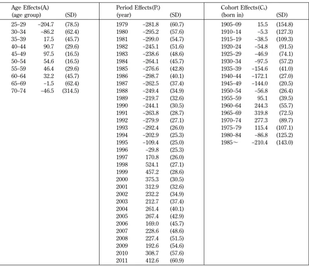
Estimation results from applying Nakamura’s method to the data in Table 5 are provided in Table 6 for 10 age groups from 25−29 to 70−74 years old and 33 annual years from 1979 to 2011. The pe-riod effects given in the middle column demonstrates “pure” time effects for 1979 to 2011, account-ing for age and cohort effects in household wine consumption.
Japanese born from 1955 to 1979, who came of age during the period of post−war prosperity, ex-hibit a greater demand for wine, all else constant. Cohort effects for this segment of the population are distinctly positive as was expected from a quick visual inspection of Table 5. However, as com-pared with consumption trends for other products such as fish and fresh fruits, the demographic ef-fects of age and generation are not as dominant a factor in determining trends in individual wine consumption (e.g., Mori and Saegusa, 2010 ; Mori, Clason, and Lillywhite, 2006 ; Mori and Stewart, 2011).
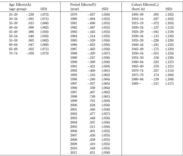
The period effects derived from the A/P/C cohort model, or “pure” time effects controlling for aging and generational replacement, seem to match very closely trends in simple average household wine consumption per adult over the survey period of 1979 to 2011, as demonstrated by Figure 1.5
For-estry, and Fisheries, 1995 ; Mori et al., 2009 ; Mori and Stewart, 2011). However, research has shown that the “pure” period effects associated with fresh fruit consumption rose slightly from 30.6 kg to 34.2kg over the corresponding period, controlling for the effects of aging and generational re-placement (e.g., Mori, Saegusa, and Dyck, 2012).
Estimation of an A/P/C model not only tests a potential explanation for trends in consumption, i. e., generational differences in tastes and preferences, but research suggests that failure to account for cohort effects in a demand model can bias estimates of price and income elasticities (e.g., Mori, Clason, and Lillywhite, 2006). Below, we consider this possibility for the case of Japanese wine de-mand. Specifically, we first estimate price and income elasticities using simple cross-sectional and time series models that ignore cohort effects. We then augment our A/P/C model with price and income variables.
5
This may not necessarily imply that it should hold true for the future.
Table 6. Individual Wine Consumption Decomposed by Age, Period, and Cohort Effects : Bayesian Estimator Model
Grand Mean Effect=597.1(9.912) (in ml)
Age Effects(Ai) (age group) (SD) Period Effects(Pt) (year) (SD) Cohort Effects(Ck) (born in) (SD) 25−29 −204.7 (78.5) 30−34 −86.2 (62.4) 35−39 17.5 (45.7) 40−44 90.7 (29.6) 45−49 97.5 (16.5) 50−54 54.6 (16.5) 55−59 46.4 (29.6) 60−64 32.2 (45.7) 65−69 −1.5 (62.4) 70−74 −46.5 (314.5) 1979 −281.8 (60.7) 1980 −295.2 (57.6) 1981 −299.0 (54.7) 1982 −245.1 (51.6) 1983 −238.6 (48.6) 1984 −264.1 (45.7) 1985 −276.6 (42.8) 1986 −298.7 (40.1) 1987 −262.5 (37.4) 1988 −249.4 (34.9) 1989 −219.7 (32.6) 1990 −244.1 (30.5) 1991 −263.8 (28.7) 1992 −279.9 (27.1) 1993 −292.4 (26.0) 1994 −202.9 (25.3) 1995 −109.4 (25.0) 1996 −29.8 (25.3) 1997 170.8 (26.0) 1998 524.1 (27.1) 1999 457.2 (28.6) 2000 375.3 (30.5) 2001 312.9 (32.6) 2002 232.2 (34.9) 2003 212.7 (37.4) 2004 261.4 (40.1) 2005 267.4 (42.9) 2006 169.0 (45.7) 2007 228.6 (48.6) 2008 227.4 (51.5) 2009 192.6 (54.6) 2010 308.7 (57.6) 2011 412.6 (60.9) 1905−09 15.5 (154.8) 1910−14 −5.3 (127.3) 1915−19 −38.5 (109.3) 1920−24 −54.8 (91.5) 1925−29 −46.9 (74.1) 1930−34 −97.5 (57.2) 1935−39 −154.6 (41.0) 1940−44 −172.1 (27.0) 1945−49 −144.0 (20.5) 1950−54 −56.8 (26.4) 1955−59 95.1 (39.5) 1960−64 244.3 (55.7) 1965−69 319.8 (72.5) 1970−74 277.3 (89.7) 1975−79 115.4 (107.1) 1980−84 −86.8 (125.2) 1985∼ −210.4 (143.0)
4. Determining Demand Elasticities for At-home Wine Consumption
FIES furnishes data on household purchases of various goods and services, including wine. The data are disaggregated by the annual income level of the households. The 1979 annual report was the last report to publish data for 18 income classes whereas the most recent annual reports only present data classified by income quintile. One can obtain, however, more detailed data for 15−18 annual income classes via CD-Roms at a library attached to the Bureau of Statistics. Below, in equa-tions (15) to (17), we report estimates of income elasticities for household wine consumption ob-tained by estimating double-log, cross-sectional regression equations using FIES data for three years, 1985, 1990, and 1995, respectively. In running the regressions, the top 1 and bottom 2 or 3 in-come classes were deleted for each year to avoid possible outliers.
First, using FIES data from only the year 1985, we find that :
log (HQi)=a+b logYi+ei (15)
=5.21+0.75 logYi
(23.6) (5.4) adj R2
=0.68
where HQiis average household wine consumption in milliliters for the i th
household income class,
Yi is average household annual income for that class in millions of yen, and ei is a random error.
The figures in parentheses denote t−values. Similarly, using FIES data from 1990, we obtain :
log (HQi)=a+b logYi+ei (16)
=5.42+0.74 logYi
(23.7) (5.5) adj R2
=0.69
Lastly, using FIES data for the year 1995, we find that :
log (HQi)=a+b logYi+ei (17)
=5.89+0.63 logYi
(34.8) (6.6) adj R2
=0.77
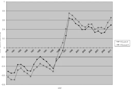
Based on the above results, it may appear safe to conclude that wine in present day Japan is a normal good, consumption of which tends to increase with income. Japan’s economy expanded very rapidly (“bubbly”) during the 1980s. However, the bubble burst in the early 1990s and the economy has subsequently experienced the “lost 20 years” (Figure 2). It is therefore curious that per−adult household wine consumption increased only moderately from 1979 to 1993, surged dramatically up to 1998, dropped abruptly up to 2002, and then stagnated, as is clearly demonstrated by Figure 1 above.6
How can we then explain these dramatic changes in household wine consumption? Income should be an important factor but changes in consumption have not seemed to follow changes in na-tional income very closely for the past three decades.
The next exercise in our analysis involved analyzing changes in household wine consumption and changes in prices using traditional time series techniques. As shown below, the first time series model we estimated was :
log Qt=a+b log Pt+et (18)
=22.56−3.35 log Pt
(13.5) (9.79) adj R2
=0.75
where Qt is per adult household wine consumption in year t in milliliters, Pt is the average real
paid price for wine in year t (2005 yen/100ml), and etis a random error. Figures in parentheses
de-note t values. The second, third, and fourth time series models we estimated were :
log Qt=a+b log Pt+c log EXPt+et (19)
18.57−3.26 log Pt+0.70 log EXPt adj. R2=0.74
(2.71) (8.60) (0.60)
log Qt=a+b log Pt+c log EXPt+dT+et (20)
27.38−0.57 log Pt−4.02 log EXPt+0.089T adj. R2=0.92
(6.79) (1.44) (0.88) (8.02)
log Qt=a+b log Pt+dT+et (21)
12.72−1.52 log Pt+0.034T adj. R2=0.86
(5.54) (3.45) (5.09)
where, additionally, EXPt is household expenditure per adult equivalence scale in year t in
mil-lions of 2005 yen and T accounts for a time trend, starting from 10 in 1979 incremented by 1 each year.
By these statistical results, average household expenditures as proxies for income have not influ-enced household wine consumption over the period from 1979 to 2011 to much extent. Average household consumption has instead been determined significantly by the prices that households faced and actually paid. The question then arises as to what degree? Average price elasticities of −3.35 and −3.26 from models (18) and (19) seem intuitively too large.7
Estimates of −0.57 from model (20) and −1.52 from model (21) appear to be more reasonable in reference to international comparisons (e.g., Wang et al., 1996, Tables 2 and 4, p. 484 and p. 487 ; Arahata, 2004, pp. 23−24 ; Fogarty, 2010, Table 2, pp. 438−448 and Table 3, p. 452) and also by the authors’ common sense. The addition of the time trend, T, in models (20) and (21) also improves statistical performance sig-nificantly. The problem is that we have neither a theoretical nor empirical justification for introduc-ing a linear time trend into our time-series demand models for wine over the period in question.
In contrast to the simple cross-sectional and time series models estimated above, several studies have incorporated income and price variables into A/P/C models. Stewart and Blisard (2008), for one, did so in their recent investigation of fresh vegetable consumption in the United States (2008, pp. 47−48). Following the lead of their study, the Japanese government research institute, PRIMAFF, introduced price and income variables into their forecast of future food expenditures in rapidly ag-ing Japan (PRIMAFF, 2010 ; Yakushiji, 2010). In the spirit of these studies, we will also try to aug-ment our Bayesian cohort model with economic variables to determine price and income elasticities of demand for household wine consumption in Japan.
When price is added to our A/P/C model for wine consumption, the average price elasticity (standard error in parentheses) is found to be −0.794 (0.421), with an accompanying AIC of −236.4 and, when the income variable is further added, average price and income elasticities are estimated at −0.798 (0.427) and −0.001 (0.006), respectively with AIC at −235.7.8
eco-nomic variables, AIC is calculated at −230.8, substantially larger than the above two cases. On the one hand, it may be statistically safe to conclude that changes in household expenditures as a proxy for income have not been a significant factor in determining trends in household wine consumption over the period of 1979 to 2011. On the other hand, we are inclined to believe that own price changes have been the dominant economic factor, with an average elasticity in the neighborhood of −0.8. We also have to admit that it is desirable to add the economic variables, at least price, to our earlier cohort analysis. The results of our augmented cohort analysis are provided in Table 7, in which all parameters are estimated in natural logs. In order to compare these results with our esti-mates of the parameters for the traditional A/P/C model without the economic variables, we again decompose the data in Table 5, in natural logs this time and provide the results in Table 8, which is therefore a log-version of Table 6.
Finally, we provide in Figure 3 a visual comparison of pure period effects in household wine con-sumption from 1979 to 2011, derived by Bayesian cohort models with and without the price variable
Table 7. Individual Wine Consumption Decomposed by Age, Period, and Cohort Effects, with Price added to the Model : Bayesian Estimator Model
Grand Mean Effect=10.085(2.057) ; Average Price Elasticity=−.794(.421) (in natural log)
Age Effects(Ai) (age group) (SD) Period Effects(Pt) (year) (SD) Cohort Effects(Ck) (born in) (SD) 25−29 −.234 (.073) 30−34 −.087 (.071) 35−39 .018 (.068) 40−44 .092 (.062) 45−49 .086 (.055) 50−54 .046 (.055) 55−59 .061 (.062) 60−64 .044 (.068) 65−69 .018 (.071) 70−74 −.044 (.073) 1979 −.514 (.073) 1980 −.553 (.100) 1981 −.554 (.087) 1982 −.367 (.095) 1983 −.364 (.094) 1984 −.408 (.097) 1985 −.494 (.097) 1986 −.508 (.082) 1987 −.361 (.077) 1988 −.255 (.083) 1989 −.195 (.073) 1990 −.252 (.073) 1991 −.300 (.077) 1994 −.378 (.077) 1995 −.448 (.091) 1994 −.282 (.089) 1995 −.203 (.086) 1996 −.058 (.072) 1997 .263 (.069) 1998 .641 (.075) 1999 .618 (.067) 2000 .525 (.059) 2001 .483 (.061) 2002 .394 (.057) 2003 .398 (.058) 2004 .459 (.056) 2005 .432 (.056) 2006 .333 (.064) 2007 .361 (.062) 2008 .314 (.074) 2009 .333 (.079) 2010 .438 (.117) 2011 .493 (.162) 1905−09 .105 (.102) 1910−14 .036 (.102) 1915−19 −.064 (.105) 1920−24 −.121 (.111) 1925−29 −.036 (.119) 1930−34 −.111 (.129) 1935−39 −.224 (.128) 1940−44 −.240 (.122) 1945−49 −.174 (.120) 1950−54 −.052 (.124) 1955−59 .154 (.125) 1960−64 .329 (.137) 1965−69 .371 (.121) 1970−74 .331 (.114) 1975−79 .167 (.106) 1980−84 −.148 (.108) 1985∼ −.322 (.117)
over the period in question. When the price variable is added to the model, the pure period effects proved slightly narrower in width than the original model but the basic periodical pattern in wine consumption as observed in Figure 2 does not change much. As discussed above, this likely repre-sents the net effects of information like reports in the 1990s that drinking red wine is healthful, in-creased sales space provided for wine by ordinary supermarkets, and other “fads and fashions”. Greater precision would require further research conducted from marketing perspectives.
6
Per adult wine consumption in terms of taxed volume more than doubled from 658ml in 1980 to 1,450ml in 1990 and kept increasing to 2,660ml in 2000 and stagnated since then to 2,600ml in 2010. At-home consumption is estimated to account for 37.1% of total wine consumption in 1980 and this share gradually dropped to 22.9%in 1990 but recovered to 35.8%in 2000 and remained at this level since then (the Japanese government National Tax Agency, 2012).
7
When simple per adult consumption, Qt, in model (19) above was replaced by the period effects, Ptfrom model (13)
in the preceding section, the average price and income elasticity are estimated at −2.98 (8.58) and 0.18 (0.17), respec-tively, with adj. R2
=0.73, as can be inferred from Figure 1.
Table 8. Individual Wine Consumption Decomposed by Age, Period, and Cohort Effects : Bayesian Estimator Model
Grand Mean Effect=6.211(.015) (in natural log)
Age Effects(Ai) (age group) (SD) Period Effects(Pt) (year) (SD) Cohort Effects(Ck) (born in) (SD) 25−29 −.239 (.073) 30−34 −.091 (.071) 35−39 .015 (.068) 40−44 .090 (.062) 45−49 .086 (.056) 50−54 .046 (.056) 55−59 .063 (.062) 60−64 .047 (.068) 65−69 .022 (.071) 70−74 −.039 (.073) 1979 −.637 (.056) 1980 −.694 (.055) 1981 −.696 (.055) 1982 −.487 (.055) 1983 −.445 (.055) 1984 −.514 (.055) 1985 −.559 (.056) 1986 −.623 (.056) 1987 −.483 (.056) 1988 −.420 (.057) 1989 −.347 (.058) 1990 −.390 (.058) 1991 −.421 (.059) 1992 −.460 (.061) 1993 −.516 (.063) 1996 −.246 (.064) 1997 −.037 (.065) 1996 .108 (.064) 1997 .407 (.062) 1998 .749 (.061) 1999 .701 (.059) 2000 .628 (.058) 2001 .560 (.058) 2002 .477 (.057) 2003 .448 (.056) 2004 .507 (.056) 2005 .511 (.056) 2006 .401 (.055) 2007 .436 (.055) 2008 .438 (.055) 2009 .410 (.055) 2010 .548 (.055) 2011 .651 (.056) 1905−09 .095 (.102) 1910−14 .027 (.102) 1915−19 −.072 (.105) 1920−24 −.127 (.112) 1925−29 −.041 (.119) 1930−34 −.115 (.130) 1935−39 −.226 (.128) 1940−44 −.241 (.122) 1945−49 −.175 (.120) 1950−54 −.051 (.124) 1955−59 .156 (.126) 1960−64 .333 (.137) 1965−69 .376 (.121) 1970−74 .337 (.114) 1975−79 .174 (.106) 1980−84 −.139 (.108) 1985∼ −.311 (.117)
8
Akaike’s Information Criteria (H. Akaike, 1980).
5. Summary and Discussions
In Japan, alcohol consumption per adult increased steadily from 1980 to the early 1990s by a little over 20% and then began to decline gradually to the 1980 level in 2010. That of sake, a traditional Japanese drink made from rice has declined persistently over the 30−year period by more than 60% to one third of the level of the early 1980s. That of beer sharply increased by more than 30% to the early 1990s and then began to decline considerably to two thirds of the level of the early 1980s in 2010. That of whisky followed a pattern similar to that of sake, whereas that of shochu rose consis-tently by 200% to 2010. At the same time, consumption of wine per adult more than tripled over the same period.
The price of sake (defined in terms of a real CPI deflated by an aggregate CPI) remained the same, whereas that of shochu rose steadily by some 20%−30% and that of beer remained more or less the same over the period of 1980 to 2010. That of whisky fell considerably in the neighborhood of 30% and the price of wine followed the same pattern as whisky over the same period.
It was found by Tanaka et al., 2004 that newer generations exhibit increasingly negative cohort ef-fects when it comes to sake consumption and older people above fifty years of age carry increas-ingly negative age effects in beer consumption. Changes in sake and beer consumption in the past three decades can largely be attributed to changes in population demographics, i.e., aging in a nar-row sense combined with the replacement of older generations by the new. What about the case of wine, which has greatly increased in consumption over the corresponding period? Our cohort analy-sis of household wine consumption has revealed that Japanese born from 1955 to 1979, who came of age during the period of post−war prosperity, exhibit the greatest demand for wine for at-home
sumption, all else constant. However, “pure time effects” have been predominant in steadily increas-ing wine consumption in the past three decades.
Failure to account for cohort effects, when present can bias estimates of price and income elastici-ties. In simple analyses of cross-sectional data that did not account for this possibility, wine con-sumption was found to be very sensitive to changes in income, with an average income elasticity estimated in the neighborhood of 0.7, using data of 8,000 households classified by some 15 income classes in 1985, 1990, and 1995, respectively. Ordinary time-series analyses of per-adult wine con-sumption from 1979 to 2011, however, did not support these findings. Japan’s national economy expanded remarkably from the end of 1970s to the early 1990s when the bubble burst and has been stagnated for the subsequent 20 years. Household wine consumption increased only moderately dur-ing the 1980s and began to surge in 1993 to the peak years of 1998−99. It then fell abruptly by 20%−30% to the early 2000s and stagnated to 2010.
The incorporation of income and price variables into an A/P/C model reveals which birth cohorts most prefer wine, i.e., Japanese born from 1955 to 1979. We also obtain reasonable income and price elasticities. The remaining “pure” period effects are hypothesized to reflect the effects of infor-mation about the healthfulness of wine consumption, the marketing efforts of various agencies con-cerned including supermarkets, and other temporal phenomena. Given the basis provided in this paper for modeling wine demand in Japan, the authors encourage further research be conducted particularly from a marketing perspective to better dissect these period effects.
References
Akaike, Hirotsugu (1980) Likelihood and the Bayesian Procedures, Bayesian Statistics (eds. J.M. Bernardo, M.H. DeGroot, D.V. Lindley and A.F.M. Smith) Valencia, University Press, 143−166. Arahata, Katsumi (2004) Market Competition among Exporting Countries and the Strategy of US
Wine, Selected Paper, the American Agricultural Economics Association Meeting, Denver, Colorado, August 1−4.
Deaton A. 1997. The Analysis of Household Surveys : A Microeconometric Approach to Development Policy, Baltimore : The Johns Hopkins University Press.
Fogarty, James (2010) The Demand for Beer, Wine and Spirits : A Survey of the Literature, Journal of Economic Survey, Vol. 24, No. 3, 428−478.
Japanese Government, Bureau of Statistics, Family Income and Expenditure Survey, various issues, Tokyo.
――Consumer Price Indexes, various issues.
――National Survey of Family Income and Expenditure, various issues. ――Library, courtesy.
Kawaguchi, Tsunemasa (1996) Professor in Agricultural Econometrics, Kyushu University, personal correspondence, Fukuoka.
Mason, W.M. and S.E. Fienberg, eds. (1985) Cohort Analysis in Social Research : Beyond the Identifi-cation Problem, New York, Springer-Verlag.
Ministry of Agriculture, Forestry and Fisheries (1995) White Paper on Agriculture for FY 1994, Tokyo, Japan.
Mori, H., D.L. Clason, and J. Lillywhite (2006) Estimating Price and Income Elasticities in the Pres-ence of Age-Cohort Effects, Agribusiness : An International Journal, 22(2), 201−217.
Mori, H. and Y. Saegusa (2010) Cohort Effects in Food Consumption : What They Are and How They Are Formed, Evolutionary and Institutional Economics Review, 7(1), 43−63.
Mori, H. and H. Stewart (2011) Cohort Analysis : Ability to Predict Future Consumption――The Cases of Fresh Fruit in Japan and Rice in Korea, Annual Bulletin of Social Science, No. 45, Senshu University, Tokyo, 153−173.
Mori, H., D. Clason, K. Ishibashi, W. Gorman, and J. Dyck (2009). Declining Orange Consumption in
Japan : Generational Changes or Something Else? U.S. Department of Agriculture, Economic
Re-search Service, Washington, D.C., Report No. 71.
Mori, H. and Y. Saegusa (2011) Estimating Demand Elasticities by Augmented A/P/C Cohort Model with the Economic Variables, Senshu Economic Bulletin, Vol. 46, No. 2, Senshu University, Tokyo, 31−53 (in Japanese).
Mori, H., Y. Saegusa and J. Dyck (2012) Estimating Demand Elasticities in a Rapidly Aging Society ――The Cases of Selected Fresh Fruits in Japan, Annual Bulletin of Social Science, No. 46, Senshu University, Tokyo, 123−144.
Nakamura, Takashi (1986) Bayesian Cohort Models for General Cohort Table Analyses, Ann. Inst. Statist. Math, 38, Part B, Tokyo, 353−370.
National Tax Agency, Statistical Report on Liquor Tax, various issues, Tokyo.
Okamoto, Masato (2003) Extension of Bayesian Cohort Models with Interaction Effects, Japanese Journal of Applied Statistics, 32(3), 145−162 (in Japanese).
PRIMAFF (2010) Outlook for Food Expenditures in a Rapidly Aging Society of Japan, Ministry of Agri-culture, Forestry and Fisheries, Tokyo (in Japanese).
Rod, M. and T. Beal (2012) The Experience of New Zealand in Evolving Wine Markets in Japan and Singapore, AAWE Working Paper, No. 100, Business, 1−18.
Sasaki, M. and T. Suzuki (1987) Changes in Religious Commitment in the United States, Holland, and Japan, American Journal of Sociology, 92(5), 1055−76.
Stewart, H. and N. Blisard (2008) Are Younger Cohorts Demanding Less Fresh Vegetables? Review of Agricultural Economics, 30(1), 43−60.
Tanaka, M., H. Mori, and T. Inaba (2004) Re-estimating per capita Individual Consumption by Age from Household Data, The Japanese Journal of Rural Economics, 6, 20−30.
Tanaka, M., H. Mori, T. Inaba and K. Ishibashi (2004) Future Projections of Household Demand for Sake and Beer ― Cohort Analysis, Quarterly Research Journal on Household Economics, No. 61, Tokyo, 50−61 (in Japanese).
Wang, J., X. M. Gao, W.J. Wailes, and G.L. Cramer (1996) U.S. Consumer Demand for Alcoholic Beverages : Cross-Section of Demographic and Economic Effects, Review of Agricultural Econom-ics, 18(3), 477−489.
Yakushiji, Tetsuro (2010) Outlook on Household Food Expenditures under the Falling Birthrate and Aging Population, Journal of Agricultural Policy Research, 18, 1−40, Tokyo (in Japanese).
Disclaimer :
1. Introduction
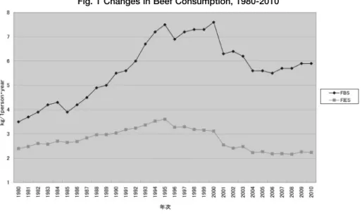
Beef consumption in Japan increased steadily from the early 1980s to the mid−1990s, due to the gradual deregulations of beef trade and the booming national economy during the 1980s. During this period, per capita consumption increased from 3.5 kg to 7.5 kg according to the Food Balance
Sheet (FBS) and per capita at-home consumption also rose from 2.4 kg to 3.6 kg according to the
Family Income and Expenditure Survey (FIES). As is shown in Fig. 1, beef consumption ceased to
grow in the mid−1990s and began to drop appreciably in the early 2000s.
E. coli O-157 was detected in selected leafy vegetables and some beef cuts in the middle of 1996
and is suspected to have adversely affected beef consumption (Oniki, 2006 ; etc.). Much more seri-ously, BSE was discovered in some beef cattle in the fall of 2001 and severely damaged the beef market across the country (Watanabe, 2004 ; Hanawa Peterson, 2005 ; alic, beef statistics ; etc.). Im-ports of grain−fed beef from North America were suspended, starting in the beginning of 2004, due to the discovery of BSE infections in cattle in the U.S. During the 10 year period since 2001, beef consumption either by FBS or FIES measures has not recovered to the mid−1990 level, approxi-mately 20% below or 35% below, respectively, in 2011.
Japan’s population has been rapidly aging during the past decades. Of approximately 8,000 house-holds (not including single person househouse-holds) covered by the FIES , those headed by under 40 year−olds and by 60 year−olds and over, respectively, accounted for 37.6 and 14.4% in 1980, 22.3 and
Part II : Estimating Impacts of the O-157 and BSE Incidents on Japanese
At-Home Beef Consumption Using an Augmented Cohort Model
Hiroshi Mori
AbstractPer capita at-home beef consumption increased steadily by 50% from the early 1980s to the mid-1990s, despite a drastic rise in away from home beef consumption. Beef consumption ceased to grow in the mid-1990s, began to decline appreciably in the early 2000s and, in the early 2010s, remains substantially below the mid-1990 level. These changes in beef consump-tion may have been caused by the booming economy during the 1980s, the steady fall in beef prices due to gradual trade liberalization in the early 1990s, changes in population struc-ture, and last but not the least the incidents of E. coli O-157 in 1996 and BSE in 2001. This paper attempts to estimate the likely impacts of these incidents on at-home beef consumption in the framework of economic and demographic change, using the A/P/C cohort model aug-mented with economic variables.
Results confirm the importance of the disease events and relative price changes for beef con-sumption in Japan.
JEL : D12, D03, Q13
27.8% in 1995 and 16.4 and 45.2%, in 2010. Beef is known to vary in individual consumption by age (Ishibashi, 2006 ; Saegusa and Mori, 2012). As is shown by Table 1, household consumption accounted for nearly 70% of total beef distribution in the late 1970s but the ratio of at-home con-sumption has been steadily declining to 37% in 2000 and to 34% by 2010. It has become increasingly common for Japanese consumers to eat beef outside the home : e.g., gyu−don (beef bowls), ham-burgers for lunch and Korean yakiniku for informal dinner since the 1970−80s. By casual observa-tions, men favor gyu-don appreciably more than women and the young, and the younger genera-tions patronize hamburger restaurants far more than the old in Japan. Regrettably, no objective data exist to substantiate these phenomena.
We will try to identify the impacts of the O−157 and BSE incidents on at-home beef consumption in Japan in the framework of demographic and economic analyses, i.e., accounting for the effects of aging and generational changes of population on the one hand and the economic factors of price and income changes on the other during the period of 1980 to 2011. The data used mainly depends on Family Income and Expenditure Survey by the Japanese government’s Bureau of Statistics, which
Table 1. Percentages of Meat Consumption by Major Outlets, 1975-2010 (%)
year 1975 1980 1985 1990 1995 1996 2000 2001 2002 2003 2008 2010 Beef At−Home 70 62 56 48 43 41 37 33 34 34 34 34 Processing 13 14 14 9 8 9 9 10 7(8) 9 6 5 Other* 17 24 30 43 49 50 54 57 59(58) 57 60 61 Pork At−Home 59 52 46 40 40 40 41 42 42 40 45 46 Processing 19 25 27 30 31 31 28 26 24(30) 29 25 25 Other 22 23 27 30 29 29 31 32 34(28) 31 30 29 Chicken At−Home 52 46 40 32 30 30 31 31 33 32 37 38 Processing 3 4 7 8 11 11 9 9 11(12) 10 8 7 Other 45 50 53 60 59 59 60 60 56(55) 58 55 55
Sources : Meat and Eggs Division, MAFF. * : Institutional and Eating Out.
classify household consumption by age groups of household-heads (HH). The model applied is the cohort analysis augmented with price and household income, designed by Saegusa (Saegusa and Mori, 2012), following the lead of Stewart and Blisard (2008, pp. 47−8).
2. Individual Beef Consumption by Age, 1980―2011 Decomposed into Age, Period
and Cohort Effects by a Traditional A/P/C Model
Individual (at-home) beef consumption by age was derived from FIES HH data from 1980 to 2011, using the Tanaka, Mori and Inaba model (2004) and is provided in Table 2. Age, period and (birth) cohort effects estimated by the Nakamura’s Bayesian estimator (Nakamura, 1986) are shown in Ta-ble 3 (in actual number of 100g) and TaTa-ble 4 (in natural log), with each effect constrained to “sum to zero”, respectively. The model (1) is an ordinary additive A/P/C equation.
μit=B+Ai+Jt+Ck+eit (1)
where
μit: average individual consumption by those of i years of age in the year, t
B : grand mean effect
Ai: age effect to be attributed to age i years old
Jt: period effect to be attributed to year t
Ck: cohort effect to be attributed to birth cohort k
eit: random error
Model (1) can be written in the conventional matrix form of a least−square regression :
Y=Xb+ε (2)
As evident in Table 2 and Table 3, those in their middle age (40s and 50s) carry positive age effects, distinctly larger than the average of zero ; age effects become gradually smaller among the older ages ; and, surprisingly, those in their 20s and 30s show a negative age effect. The older cohorts born before the mid-1930s, who came of age during the food shortage era, when per capita meat supply was less than 2−3 kg per year on average, have a negative cohort effect ; those born during the 1940−1970 period have a clearly positive cohort effect ; but those newer cohorts born after the mid-1980s show an increasingly negative cohort effect as the birth years become more recent. It should be kept in mind that the data used, Table 2, relate to at−home consumption alone and beef eaten in McDonald’s or Yoshinoya (gyu-don restaurants) is not counted.
Using these “pure” or net time effects with the demographic effects of aging and cohort-replacement of population accounted for, we next regress our estimates of annual period effects against the economic factors : changes in prices and income over the period in question.
(B+Jt)=a+b log(RBFPt)+c log(REXt)+et (3)
=−12.16+0.64 log(RPPt)+2.35 log(REXt)
(2.43) (2.40) (3.16) Adj. R2
=0.205 B: grand mean effect (3.319, Table 4)
Jt: period effect for year t (Table 4)
RBFPt: real average paid price of fresh beef in year t (yen/100 g : base year=2005)
REXt: real living expenditure/adult equivalence*in year t (10 thousand yen : base year=2005)
* Oxford equivalence scale (=“old OECD scale” : OECD, 2009) Number in parentheses : t value
Model (3) is questionable because the coefficient for own price, c proved positive. We will then introduce the price of the competing meats, weighted average prices of fresh pork and chicken in model (4) below.
(B+Jt)=a+b log(RBFPt)+c log(REXt)+d log(RPCPt)+et (4)
=−27.79−0.45 log(RBFPt)+4.37 log(REXt)+2.39 log(RPCPt)
(6.55) (1.77) (7.27) (6.03) Adj. R2
=0.642 RPCPt : real average paid price
1
of fresh pork and chicken in year t (yen/100 g : base year=2005)
Table 2. Changes of At-Home Individual Beef Consumption by Age, 1980-2011 (100g/year)
15−19 20−24 25−29 30−34 35−39 40−44 45−49 50−54 55−59 60−64 65−69 70−74 75+ 1980 23.66 23.75 22.79 27.01 29.72 31.37 30.03 35.47 29.05 26.04 24.55 21.91 18.63 1981 24.58 22.48 20.50 28.81 31.99 32.57 37.88 37.23 33.16 22.15 22.44 20.83 17.95 1982 27.14 26.47 25.17 28.67 31.94 33.65 34.24 36.75 33.00 26.33 23.67 20.64 17.41 1983 26.65 25.09 23.63 27.19 33.19 31.59 38.09 35.77 35.91 27.05 23.07 19.53 16.25 1984 27.42 24.13 22.31 28.23 30.19 38.73 35.18 37.07 33.94 30.96 27.63 23.99 20.09 1985 29.61 25.65 22.23 26.69 29.54 34.05 39.40 35.75 31.22 30.22 26.52 22.88 19.09 1986 29.17 25.49 22.76 26.56 31.38 34.31 38.38 34.89 33.38 32.21 26.92 22.47 18.42 1987 30.21 26.64 23.98 28.51 32.59 38.69 43.04 39.66 40.10 28.94 24.26 20.57 17.16 1988 30.94 26.59 23.12 28.91 32.29 43.37 40.38 40.62 36.43 30.81 27.89 24.52 20.69 1989 33.17 28.85 24.96 27.65 32.84 38.75 42.42 38.95 34.46 34.47 29.58 25.22 20.82 1990 32.81 29.63 26.62 31.69 34.60 38.29 43.93 41.52 35.07 35.43 27.68 22.34 17.98 1991 33.23 30.68 28.22 32.12 35.58 40.80 44.49 43.34 39.92 35.00 31.70 27.81 23.38 1992 37.18 35.88 33.89 30.25 34.33 39.56 40.75 39.17 41.73 34.54 30.43 26.27 21.91 1993 36.81 33.80 29.30 31.60 36.69 41.86 50.26 47.09 38.15 37.18 33.11 28.86 24.20 1994 37.82 33.50 28.97 34.79 37.74 48.60 50.75 49.76 40.20 39.66 32.56 27.10 22.26 1995 38.16 35.26 31.81 34.74 39.63 46.09 51.65 50.12 44.04 41.89 32.67 26.36 21.36 1996 37.55 34.75 32.18 30.41 31.59 41.02 43.99 40.34 43.18 35.34 30.54 26.27 21.90 1997 35.84 32.53 29.29 28.47 34.61 42.55 44.99 42.82 43.18 38.27 32.77 27.87 23.07 1998 34.45 32.53 29.82 29.18 30.63 42.87 41.01 43.72 39.87 36.86 30.70 25.60 21.04 1999 30.98 27.84 25.27 29.60 31.52 42.99 42.69 44.18 41.38 37.78 33.75 29.24 24.40 2000 33.52 30.34 26.77 26.49 31.36 39.91 43.27 42.22 39.76 35.27 31.74 28.57 24.28 2001 29.46 27.37 24.55 21.67 24.37 31.85 34.62 33.59 32.33 29.52 25.73 21.45 17.48 2002 26.22 25.21 23.18 21.66 23.93 29.45 32.67 33.51 31.74 27.34 23.88 21.06 17.82 2003 24.78 23.16 21.99 22.13 25.10 30.23 31.77 30.89 32.01 32.44 29.51 24.50 19.82 2004 20.07 19.17 17.84 18.38 21.68 27.11 30.50 31.93 31.48 28.71 26.14 23.54 20.08 2005 17.87 16.15 14.27 17.56 22.83 28.98 32.99 34.69 33.16 28.79 26.23 24.53 21.35 2006 20.11 19.19 17.96 18.24 21.21 26.28 29.19 30.16 30.02 27.92 25.38 22.45 18.95 2007 17.32 16.22 15.28 17.41 21.46 26.82 30.02 31.40 32.07 30.59 27.25 22.87 18.77 2008 17.58 16.73 15.91 16.38 19.89 25.95 29.17 30.25 31.75 31.58 28.46 23.60 19.18 2009 18.03 18.02 17.79 18.88 21.84 26.49 29.92 32.21 33.49 32.21 28.52 23.57 19.21 2010 19.06 17.39 16.10 16.65 20.78 27.73 30.55 30.47 32.09 32.67 29.34 23.74 18.96 2011 17.27 16.79 16.65 18.36 21.42 25.46 27.85 29.07 30.78 31.00 28.58 24.46 20.22
1Constant weights of 2 to 1 are applied to pork and chicken in deriving average prices.
By adding the aggregate price of pork and chicken to the model, we have obtained a seemingly reasonable own price elasticity, in respect of sign and magnitude. The elasticity of substitution car-ries the right sign but may be too large in magnitude (M. Sawada, 2012, p. 191). More troublesome is that the estimated expenditure elasticity, 4.4, appears to be far too large (Obara, McConnel, and Dyck, 2010, pp. 13−14 ; Saegusa and Mori, 2012 ; also see subsequent footnote 2).
As mentioned above, the beef market in Japan underwent two major incidents : O-157 in the mid− 1990s and BSE in the early 2000s. Therefore, we introduce dummy variables into our regression model, to represent these incidents. We first incorporate a dummy for BSE.
(GM+Jt)=a+b log(RBFPt)+c log(REXt)+d log(RPCPt)+f I1BSE+et (5)
=−4.08−0.29 log(RBFPt)+1.42 log(REXt)+0.40 log(RPCPt)−0.287*I1BSE
(1.67) (2.95) (4.41) (1.88) (12.93) Adj. R2
=0.948
Table 3. Individual At-home Beef Consumption Decomposed into Age/ Period/ Cohort Effects by Bayesian Estimator
Grand Mean Effect=28.98(0.22) (100g/1 person)
Age Effects Age (SD) Period Effects Year (SD) Cohort Effects Born in (SD) 15−19 −1.06 1.14 20−24 −3.95 1.15 25−29 −6.80 1.20 30−34 −5.19 1.24 35−39 −2.05 1.35 40−44 3.52 1.49 45−49 6.15 1.49 50−54 5.95 1.35 55−59 4.53 1.24 60−64 2.31 1.20 65−69 −0.31 1.15 70−74 −3.11 1.14 1980 −2.08 0.80 1981 −1.43 0.78 1982 −0.57 0.78 1983 −0.51 0.78 1984 0.24 0.77 1985 −0.09 0.76 1986 0.23 0.76 1987 1.51 0.78 1988 2.19 0.80 1989 2.62 0.83 1990 3.31 0.86 1991 4.85 0.88 1992 5.19 0.88 1993 6.62 0.89 1994 7.84 0.90 1995 8.28 0.91 1996 5.32 0.91 1997 5.22 0.90 1998 4.11 0.89 1999 3.81 0.89 2000 2.66 0.89 2001 −2.38 0.86 2002 −3.98 0.83 2003 −3.80 0.80 2004 −5.83 0.78 2005 −6.01 0.76 2006 −6.64 0.76 2007 −6.59 0.77 2008 −6.51 0.78 2009 −5.58 0.78 2010 −5.75 0.78 2011 −6.28 0.80 1906−10 −3.31 2.11 1911−15 −3.52 2.12 1916−20 −3.90 2.14 1921−25 −4.10 2.14 1926−30 −2.44 2.08 1931−35 −0.24 1.97 1936−40 1.30 1.87 1941−45 3.02 1.74 1946−50 4.49 1.68 1951−55 4.52 1.67 1956−60 3.31 1.71 1961−65 1.52 1.89 1966−70 0.46 2.08 1971−75 1.20 2.00 1976−80 1.75 2.07 1981−85 1.67 2.15 1986−90 0.35 2.14 1991−95 −2.42 2.14 1996∼ −3.64 2.16
Source : Calculated by the author using the data provided in Table 2.
I1 : Indicator variable for BSE=1, if t>2000
The addition of a BSE dummy improved the model’s statistical performance and the parameter es-timates for own price and substitution and expenditure elasticities look reasonable. We next add a dummy for O-157, thought to have damaged beef consumption relatively less than BSE (Ishibashi, 2012).
(GM+Jt)=a+b log(RBFPt)+c log(REXt)+d log(RPCPt)+f I1BSE+gI2O-157+et (6)
=−1.92−0.56log(RBFPt)+1.27log(REXt)+0.45log(RPCPt)−0.341*I1BSE−0.112*I2O-157
(6.89) (8.51) (6.89) (3.66) (23.49) (7.57) Adj. R2
=0.983 I1 : Indicator variable for BSE=1, if t>2000
I2 : Indicator variable for O−157=1, if t>1995, <2001
The model fit is further improved by adding O-157 and all the parameter estimates look more rea-sonable with much higher t-values than model (5). In assigning the indicator variable for BSE, we
Table 4. Individual At-home Beef Consumption Decomposed into Age/Period/Cohort Effects by Bayesian Estimator
Grand Mean Effect=3.319(0.008) (in natural log)
Age Effects Age (SD) Period Effects Year (SD) Cohort Effects Born in (SD) 15−19 −0.170 0.071 20−24 −0.136 0.059 25−29 −0.257 0.047 30−34 −0.195 0.035 35−39 −0.077 0.023 40−44 0.101 0.014 45−49 0.180 0.014 50−54 0.188 0.023 55−59 0.162 0.035 60−64 0.103 0.047 65−69 0.026 0.059 70−74 −0.077 0.284 1980 −0.047 0.043 1981 −0.035 0.041 1982 −0.001 0.039 1983 −0.002 0.037 1984 0.024 0.034 1985 0.014 0.032 1986 0.023 0.030 1987 0.054 0.028 1988 0.078 0.026 1989 0.096 0.025 1990 0.115 0.023 1991 0.160 0.021 1992 0.174 0.020 1993 0.207 0.019 1994 0.234 0.018 1995 0.243 0.018 1996 0.174 0.018 1997 0.168 0.018 1998 0.138 0.019 1999 0.126 0.020 2000 0.090 0.021 2001 −0.062 0.023 2002 −0.118 0.025 2003 −0.116 0.026 2004 −0.198 0.028 2005 −0.220 0.030 2006 −0.230 0.032 2007 −0.239 0.034 2008 −0.235 0.037 2009 −0.195 0.039 2010 −0.202 0.041 2011 −0.218 0.043 1906−10 −0.156 0.118 1911−15 −0.164 0.104 1916−20 −0.161 0.093 1921−25 −0.140 0.080 1926−30 −0.064 0.068 1931−35 0.002 0.055 1936−40 0.054 0.043 1941−45 0.108 0.031 1946−50 0.159 0.022 1951−55 0.175 0.017 1956−60 0.149 0.021 1961−65 0.104 0.030 1966−70 0.070 0.041 1971−75 0.085 0.053 1976−80 0.079 0.066 1981−85 0.047 0.079 1986−90 −0.018 0.092 1991−95 −0.138 0.104 1996∼ −0.190 0.115
first gave 0.3 for year 2001 and 1 for 2002, and 0 afterwards, since BSE was discovered in Septem-ber 2001 and the market disruption is reported to have calmed down before the beginning of 2003 (Watanabe, 2004), which did not result in appreciable improvement from model (4), without a BSE dummy. We then assigned 1 to 2003, and 0 afterwards ; then another 1 to 2004 ; ――, to reach the best result, model (6). This process could be technically enhanced by “piece−wise linear regression” (Pindyck and Rubinfeld, 1981), for example.
A brief interpretation of model (6) above concerning the impacts of BSE and O-157, respectively is presented here. Average per capita consumption in 1995 is estimated from Table 4 as exp(3.319+ 0.243)=exp(3.562)=35.23(100 g). As a coefficient for O-157 is determined at −0.112, average con-sumption after the incident could be estimated as exp(3.562−0.112)=exp(3.450)=31.50(100 g) in ac-tual value, i.e., per capita consumption should have dropped by (35.23−31.50)=3.73(100 g) as a pos-sible consequence of the O-157 incident. Similarly, theoretical per capita consumption in the year 2000=exp(3.319+0.090)=exp(3.409)=30.23. When a BSE coefficient=−0.341 is added, theoretical consumption is estimated as exp(3.409−0.341)=exp(3.068)=21.50(100 g) in actual value, i.e., per capita consumption should have dropped by (30.23−21.50)=8.73(100 g), as a possible consequence of the BSE incident.
We learned recently that a traditional A/P/C model could encounter some structural problems in identifying cohort parameters, period effects in particular, when a time trend in consumption is se-verely hampered by abrupt, irregular market forces, for example, “fads and fashion” in the case of wine in Japan (Rod and Beal, 2012) or the BSE incident in beef (Saegusa and Mori, 2012). We will replicate in the subsequent section the analysis undertaken in this section, using “augmented” co-hort model with price and income pre-installed.
3. Decomposing Individual At-home Beef Consumption by Age by a New Cohort
Model, “Augmented” with Price and Household Income
μit=B+Ai+Jt+Ck+c RBPPt+d REXPt+eit (7)
where
all the data are logarithmic
RBPPt: real average paid price of beef in year t
REXPt: real living expenditure/adult equivalence in year t
c : constant price elasticity d : constant expenditure elasticity
The results are provided in Table 5, which demonstrates that the “net” time effects are gradually declining to the mid-1990s and then dropped suddenly in 1996 and again sharply in 2001, with the effects of changes in price and household income over the entire period accounted for2
. We suspect that these two abrupt drops in the period effect should represent possible impacts of O-157 and BSE, respectively, on individual at−home beef consumption.
When converted into actual numbers in 100 g per year (the 2nd
Table 5. Individual At-Home Beef Consumption Decomposed into Age/Period/Cohort Effects by Bayesian Estimator Augmented by Price and Income
Grand Mean Effect=3.321(0.008) (in natural log)
Est. Price Elast.=−0.559(0.213) ; Est. Expenditure Elast.=0.839(0.592)
Age Effects Age (SD) Period Effects Year (SD) Cohort Effects Born in (SD) 15−19 0.020 0.041 20−24 −0.106 0.042 25−29 −0.233 0.043 30−34 −0.178 0.045 35−39 −0.066 0.049 40−44 0.104 0.054 45−49 0.177 0.054 50−54 0.177 0.049 55−59 0.145 0.045 60−64 0.079 0.043 65−69 −0.004 0.042 70−74 −0.115 0.041 1980 0.177 0.075 1981 0.170 0.076 1982 0.175 0.070 1983 0.157 0.064 1984 0.160 0.060 1985 0.145 0.055 1986 0.145 0.050 1987 0.154 0.049 1988 0.148 0.053 1989 0.151 0.055 1990 0.150 0.054 1991 0.159 0.050 1992 0.139 0.049 1993 0.125 0.047 1994 0.115 0.042 1995 0.110 0.041 1996 0.048 0.040 1997 0.048 0.039 1998 0.022 0.038 1999 0.003 0.036 2000 −0.041 0.034 2001 −0.173 0.034 2002 −0.218 0.032 2003 −0.192 0.031 2004 −0.230 0.031 2005 −0.240 0.030 2006 −0.233 0.034 2007 −0.240 0.033 2008 −0.229 0.039 2009 −0.216 0.045 2010 −0.241 0.043 2011 −0.245 0.043 1906−10 −0.102 0.076 1911−15 −0.110 0.077 1916−20 −0.112 0.078 1921−25 −0.099 0.078 1926−30 −0.029 0.075 1931−35 0.029 0.072 1936−40 0.074 0.068 1941−45 0.122 0.063 1946−50 0.166 0.061 1951−55 0.175 0.060 1956−60 0.143 0.062 1961−65 0.090 0.068 1966−70 0.050 0.076 1971−75 0.058 0.073 1976−80 0.045 0.075 1981−85 0.006 0.078 1986−90 −0.065 0.078 1991−95 −0.191 0.077 1996∼ −0.249 0.078
Sources and Notes : the same as Table 3.
2The own price and expenditure elasticities are determined at−0.56 and 0.84, respectively (on the upper part, Table 5),
which seem to be realistic (see Obara, McConnel, and Dyck, op. cit. and Saegusa and Mori, op. cit.). Concerning in-come elasticities of household demand for beef, we conducted cross-sectional analyses of FIES data, classified by 17− 18 income classes in 1985 and 1995, to obtain the average elasticities of 0.7 to 0.8.
log (capQi)=a+b log(EXi)+e (8)
1985 : =−0.548+0.79 log(EXi)
(2.08) (14.42) AdjR2=0.963 1995 : =0.080+0.69 log(EXi)
(0.26) (11.15) AdjR2=0.925 where
capQi: per capita beef purchase (100g) by ithhousehold by annual income class
the incident of O-157. The same consumption base is estimated as exp (3.321−0.041)=26.58(100 g) in 2000, which fell to exp (3.321−0.173)=23.29 in 2001 and exp (3.321−0.218)=22.26 in 2002, by approximately 400 g. These abrupt decreases could be attributed to the incident of BSE, which occurred in the fall of 2001 in Japan.
The “theoretical base” of at-home beef consumption then declined a little further to exp (3.321− 0.240)=21.78(100 g) in 2005 and stayed virtually unchanged to 2011 (Fig. 2). What may call for at-tention is that the consumption base of Japanese at−home beef consumption has not recovered to the mid-1990s’ level, whether due to persisted impacts of O-157 and BSE incidents and/or some other factors.
Japanese beef has been characterized as very expensive by international standards (Hayami, 1979 ; Longworth, 1983 ; Coyle, 1986 ; etc.). Japanese beef has become substantially cheaper since the early 1980s, because of the freer trade and appreciably stronger yen against the U.S. and Austra-lian dollars (Mori and Gorman, 1995). And yet, beef is much more expensive than other meats, a lit-tle more than twice as high as pork, and three times higher than chicken in Japan at present. In a long-stagnated economy, Japanese consumers have been shifting from beef to cheaper meats (alic, Research Department, 2012). Mainly due to the suspension of grain−fed beef imports from North America, the average retail price of fresh beef increased nearly 20% from 2000 to 2008, whereas that of pork and chicken kept unchanged. At-home, Japanese consumers ate nearly 10% more meats in 2011 than in 2000. As is shown in Table 6, household purchases of beef decreased from 10.1 kg in 2000 to 6.8 kg in 2011, whereas that of pork increased from 16.0 to 19.0 kg and that of chicken rose from 11.6 to 13.7 kg during the same period. Our research provides strong indications that shocks from the O-157 and BSE incidents as well as the changes of beef price relative to substitutes, were responsible for some of the decline in at−home beef consumption. Our results also show that, for at-home consumption, young people consume below-average amounts of beef. Further research about beef consumption by young people away from home is needed to determine whether the preference for beef will decline in the future.
References
alic, Research Department (2012) Personal Correspondence, Summer.
Coyle, William T. (1986) The 1984 U.S.−Japan Beef and Citrus Understanding : An Evaluation, USDA, Economic Research Service, Foreign Agricultural Economic Report No. 222.
Hanawa Peterson, H. and Chen Y−J (2005) “The Impact of BSE on Japanese Retail Meat Demand,” Agribusiness : an International Journal, 21(3), 313−327.
Hayami, Yujiro (1979) “Trade Benefits to All : A Design of the Beef Import Liberalization in Japan,” American Journal of Agricultural Economics, 61(2), 342−347.
Ishibashi, Kimiko (2006) Demographic Analysis of Japanese Food Consumption by Age and Household Types, National Agricultural Research Center, Tsukuba (in Japanese).
―― (2012) Personal communications, formerly Senior Researcher at National Center for Agricul-tural Research, Tsukuba.
Japanese Government, Bureau of Statistics, (Annual Report) Family income and Expenditure Survey, various issues.
Japanese Government, Policy Research Institute, Ministry of Agriculture and Forestry and Fisheries PRIMAFF (2010) Outlook for Food Expenditures in Rapidly Aging Society of Japan, Tokyo (in Japa-nese). <http://www.maff.go.jp/j/press/kanbo/kihyo01/100927.html>
Longworth, John (1983) Beef in Japan : Politics, Production, Marketing and Trade, University of Queensland Press, St. Lucia, Queensland.
Mori, H. and Wm. D. Gorman (1995) “The Japanese Beef Market Following Liberalization : What Has and Has not Happened?” Journal of Rural Economics, 67(1), 20−30.
Mori, H. and D.L. Clason, and J. Lillywhite (2006) “Estimating Price and Income Elasticities for Foods in the Presence of Age−Cohort Effects,” Agribusiness : an International Journal, 22(2), 201− 17.
Mori, H., D. Clason, K. Ishibashi, Wm. D. Gorman, and J. Dyck (2009) Declining Orange
Consump-tion in Japan : GeneraConsump-tional Changes or Something Else? Economic Research Report No. 71, ERS,
Table 6. Household Purchases of Beef, Pork and Chicken, 2000-2011
Beef Pork Chicken
Quantities Paid Prices Quantities Paid Prices Quantities Paid Prices
kg/year yen/100g index kg/year yen/100g index kg/year yen/100g index
2000 10.099 258.84 100.0 16.040 134.33 100.0 11.591 91.49 100.0 2001 8.205 257.49 99.5 16.341 135.45 100.8 11.644 92.80 101.4 2002 7.694 260.94 100.8 17.010 136.80 101.8 12.061 94.56 103.4 2003 7.963 270.07 104.3 16.365 133.55 99.4 11.618 92.27 100.9 2004 7.113 296.66 114.6 17.335 135.16 100.6 10.944 93.03 101.7 2005 7.195 296.38 114.5 17.407 133.23 99.2 11.647 92.29 100.9 2006 6.891 300.45 116.1 17.305 134.35 100.0 11.985 90.70 99.1 2007 6.869 303.82 117.4 17.723 134.98 100.5 12.379 91.24 99.7 2008 6.776 308.24 119.1 18.310 139.57 103.9 12.661 101.33 110.8 2009 7.032 286.8 110.8 18.639 133.00 99.0 13.647 92.44 101.0 2010 6.922 273.98 105.8 18.498 129.51 96.4 13.753 90.06 98.4 2011 6.782 274.15 105.9 18.987 130.30 97.0 13.702 93.43 102.1
USDA.
Mori, H., Y. Saegusa and J. Dyck (2012) “Estimating Demand Elasticities in a Rapidly Aging Society ――The Cases of Selected Fresh Fruits in Japan,” Annual Bulletin of Social Science, No. 46, Sen-shu University, 123−144.
Nakamura, Takashi (1986) “Bayesian Cohort Models for General Cohort Tables,” Annals of the Insti-tute of Statistical Mathematics, 38, 353−370,
Obara, K., M. McConnel, and J. Dyck (2010) Japan’s Beef Market, LDP−M−194−01, Economic Re-search Service, USDA.
OECD (2009) OECD Project on Income Distribution and Poverty, Paris.
Oniki, Shunji (2006) “Valuing Food−Born Risks Using Time−Series Data : The Case of E. coli O 157 : H7 and BSE Crises in Japan,” Agribusiness : an International Journal, 22(2), 219−32.
Pindyck, R.S. and D.L. Rubinfeld (1981) Econometric Models and Economic Forecasts, McGraw-Hill Book Company, New York.
Rod, M. and T. Beal (2012) “The Experience of New Zealand in the Evolving Wine Markets of Ja-pan and Singapore,” Working Paper, No. 100, Business, JWE, American Association of Wine Eco-nomics, 1−18.
Saegusa, Y. and H. Mori (2012) “Estimating Demand Elasticities by Augmented Cohort Model−the Cases of Beef and Wine, Economic Bulletin of Senshu University, 47(1), 1−22 (in Japanese).
Sawada, Manabu (2012) “Structural change in Japanese household demand for fresh meat in the 1990s,” FOOD CONSUMPTION−Empirical Studies of Japanese Dietary, edited by Kozo Sasaki, Tsukuba−shobo, Tokyo.
Stewart, H. and N. Blisard (2008) “Are Younger Cohorts Demanding Less Fresh Vegetables?” Re-view of Agricultural Economics, Vol. 30, No. 1, 43−60.
Tanaka, M., H. Mori and T. Inaba (2004) “Re−estimating per Capita Individual Consumption by Age from Household Data,” Japanese Journal of Rural Economics, Vol. 6, 20−30.
Watanabe, Noriyuki (2004) “Recent Trends in Meat Consumption in Household Surveys,” Agricul-ture and Livestock Industry Promotion Corporation (in Japanese).