Motion Planning and Control for a Class of Underactuated Systems

(1)

九州大学学術情報リポジトリ

Kyushu University Institutional Repository

Motion Planning and Control for a Class of Underactuated Systems

白, 楊

http://hdl.handle.net/2324/2236225

出版情報：九州大学, 2018, 博士（工学）, 課程博士バージョン：

権利関係：

(2)

2019 Doctoral Thesis

MOTION PLANNING AND CONTROL FOR A CLASS OF UNDERACTUATED SYSTEMS

Control Engineering Lab.

Department of Mechanical Engineering, Kyushu University D3 Yang BAI

2019. 1. 10

(3)

Acknowledgements

My thesis is completed with a lot of help from many people during my doctor study at Kyushu University.

First I would like to sincerely thank Professor Mikhail Svinin for all his help in my research. His insightful guidance, kind encouragement, and patience have been great support throughout my research and strengthened my goal to be a researcher.

At the same time, I would like to thank Professor Motoji Yamamoto for his great help in my research and graduation.

Also I would like to thank Professor Kazuo Kiguchi, Professor Shinji Hokamoto, and Professor Ryo Kurazume for there suggestions and comments to my thesis.

I am also thankful to Professor Ryo Kikuuwe, Professor Kenji Tahara and Professor Yasutaka Nakashima for their valuable comments.

Finally, I am deeply thankful to my family. Their encouragement and expectation support and inspire me to work hard on my research.

(4)

List of figures

1.1 Inner-wheel-driven rolling robot . . . 3

1.2 Deformable type rolling robot . . . 4

1.3 Rotor-driven rolling robot . . . 4

1.4 Pendulum-driven rolling robot . . . 5

2.1 Ball-pendulum system formalization. . . 13

2.2 Definition of basic vectors. . . 15

2.3 Motion planning problem. . . 19

2.4 Spherical robot tracing given contact path. . . 23

2.5 Hoop-pendulum system. . . 25

2.6 Motion pattern for the base variableθ(t) . . . 29

2.7 Hoop motions resulted from geometric phase based control. . . 31

2.8 Pendulum motions resulted from geometric phase based control. . . 31

2.9 Relation betweenθ_mandφ_desfor the hoop-pendulum system under the geometric phase based motion planning algorithm. The yellow and red portions of the curve illustrate this relation respectively whenφ_desis rather small and large. . . 32

2.10 Displacement and velocity of the shell alongX-axis (red curve) and along Y-axis (blue curve). . . 37

2.11 Generalized coordinates of the pendulumq1,q˙1 (red curve) andq2, q˙2 (blue curve). . . 37

2.12 Generalized accelerations and torques on the pendulum: q¨₁, τ₁ (red curve) andq¨₂,τ₂ (blue curve). . . 37

(8)

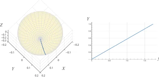
2.13 Trace of the contact point on the spherical surface (left) and on the plane (right). . . 38 2.14 Displacement and velocity of the shell alongX-axis (red curve) and along

Y-axis (blue curve). . . 38 2.15 Generalized coordinates of the pendulumq₁,q˙₁ (red curve) andq₂, q˙₂ (blue

curve). . . 39 2.16 Generalized accelerations and torques on the pendulum: q¨1, τ1 (red curve)

andq¨₂,τ₂ (blue curve). . . 39 2.17 Trace of the contact point on the spherical surface (left) and on the plane

(right). . . 39 2.18 Displacement and velocity of the shell alongX-axis (red curve) and along

Y-axis (blue curve). . . 40 2.19 Generalized coordinates and angular velocities of the pendulum q1, q˙1 (red

curves) andq₂,q˙₂ (blue curves). . . 41 2.20 Generalized accelerations and torques on the pendulum: q¨₁, τ₁ (red curve)

andq¨₂,τ₂ (blue curve). . . 41 2.21 Trace of the contact point on the spherical surface (left) and on the plane

(right). . . 41 2.22 Displacement and velocity of the shell alongX-axis (red curve) and along

Y-axis (blue curve). . . 42 2.23 Generalized coordinates and angular velocities of the pendulum q₁, q˙₁ (red

curves) andq₂,q˙₂ (blue curves). . . 42 2.24 Generalized accelerations and torques on the pendulum: q¨₁, τ₁ (red curve)

andq¨2,τ2 (blue curve). . . 43 2.25 Trace of the contact point on the spherical surface (left) and on the plane

(right). . . 43 2.26 Motion of the ball-pendulum system under non-adaptive control. . . 53 2.27 Motion of the ball-pendulum system under the FAT-based adaptive control. 54 3.1 A closed loop in shape variables producing a displacement in the fiber vari-

able. . . 60

(9)

3.2 Motion pattern of the based variableqb(t) . . . 65

3.3 Cart-pole system . . . 68

3.4 Motion of the cart-pole system resulted from the geometric phase based control. . . 70

3.5 Motion of the cart-pole system resulted from the minimum effort optimal control. . . 70

3.6 Planar ballbot system. . . 72

3.7 Motion of the ballbot system resulted from the geometric phase based control. 74 3.8 Motion of the ballbot system resulted from the minimum effort optimal control. . . 74

4.1 System response of double integrator under constructed controller. . . 88

4.2 Input signal. . . 88

4.3 Nonlinear system response under constructed controller. . . 91

4.5 Unicycle system. . . 92

4.6 Nonlinear system response under constructed controller. . . 95

5.1 A process of the neural network aided FAT approach to controller design for robots. . . 102

5.2 Swarm control of spherical robots for mapping of an indoor environment. . 103

5.3 Definition of basic vectors with respect to the planeP. . . 116

(10)

List of tables

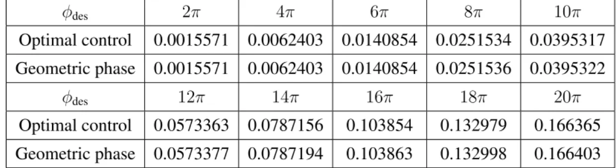
2.1 Comparison for the values of the cost functionJ, expressed by (2.30), between the minimum effort optimal control formulation and the geometric phase based approach for the hoop-pendulum system. . . 32 3.1 Comparison for the values of the cost functionJ, expressed by (2.30), be-

tween the minimum effort optimal control formulation and the geometric phase based approach for the cart-pole system. . . 71 3.2 Comparison for the values of the cost functionJ, expressed by (2.30), be-

tween the minimum effort optimal control formulation and the geometric phase based approach for the ballbot system. . . 75

(11)

Chapter 1 Introduction

1.1 Background

In recent years there has been a growing interest to the motion planning and control of underactuated mechanical systems [2–5]. These systems have fewer independent actuators than the number of degrees of freedom. The need for analysis and control of underactuated mechanical systems arises in many practical applications that include the use of ships, underwater vehicles, helicopters, aircraft, satellites, space platforms,mobile robots, flexible joint robots, hyper-redundant and snake-like manipulator, walking robots, capsule robots, and hybrid machines [2–5].

The underactuated systems are superior to the fully actuated systems in terms of energy saving, cost reduction, weight reduction, and system flexibility. Also, the simple structure of underactuated system facilitates overall kinetic analysis and planning. At the same time, due to the high nonlinearity of the system, the underactuated system is complex enough to verify the effectiveness of various algorithms. In the practical implementation, a fully actuated system, when part of the driving mechanism fails, may become an underactuated system, and the control algorithm developed for underactuated systems can play a role of fault-tolerant control.

Despite these merits, from the perspective of control theory, the limitation of the input for the underactuated system leads to challenging planning and control problems: the un-

(12)

deractuated portion of the system dynamics forms a nonholonomic constraint between the output variables. The planned and the controlled trajectories for these variables need to respect this constraint.

This thesis seeks to provide motion planning and control methods for a class of underactuated systems. Before tackling this generic problem, I first start from a specific type of underactuated system, the spherical rolling robot, to demonstrate the features of underactuated systems, as well as the corresponding difficulties in the motion planning and control.

Then, based on the study of this specific problem, I extend our methods to more generic problems, motion planning and control for a class of underactuated systems. The detailed introductions for each topic (spherical rolling robot, motion planning and control for underactuated systems) are as follows.

1.1.1 Spherical rolling robots

Spherical rolling robots are a special type of mobile robots, the image of which can be seen in many recent movies, such the Star Wars and the Jurassic World. Different from the vast majority of mobile robots that either have legs or exploit conventional multiple wheels, the spherical rolling robots, considered as single wheel vehicles, represent a new type of mechanical systems demonstrating rich and intriguing dynamics.

The first self-propelled spherical robot can be traced back to the 1900s. The rolling robot was driven by a gyroscope inside and the dynamic model was verified under experiments.

However, the main issue of the study on the spherical robot is the integrability of motion equations, and no notion of control is involved in the analysis. Only in the last two decades there appeared studies in the control area on problems of motion planning and trajectory tracking of spherical robot. Meanwhile, rolling robots have also been introduced to applications such as surveillance, inspection, guarding, and disaster mitigation. Robotic toys for the education, sport and entertainment industries are also in this group.

Motivations behind the research and applications are the advantages of spherical rolling robots compared other types of mobile robots. The advantages of spherical rolling robots can be seen from the following aspects. First is their omnidirectional mobility. They can rotate along any desired direction. This ability enables spherical robots to pass around obstacles in

(13)

minimum effort. Second is its geometric symmetry. This characteristic endows the spherical robot with the robustness that it can start or stop at any position and will never fall down or be turned upside down as other mobile robot such as wheeled robot or legged robot do. Also it should be noted that all the devices of the spherical robot are covered by its outer shell.

Therefore its driving mechanisms and its sensors are very well protected when rotating, bouncing or working under special condition such as uneven terrain or under water.

Encouraged by these advantages, many designs of spherical robots have been proposed.

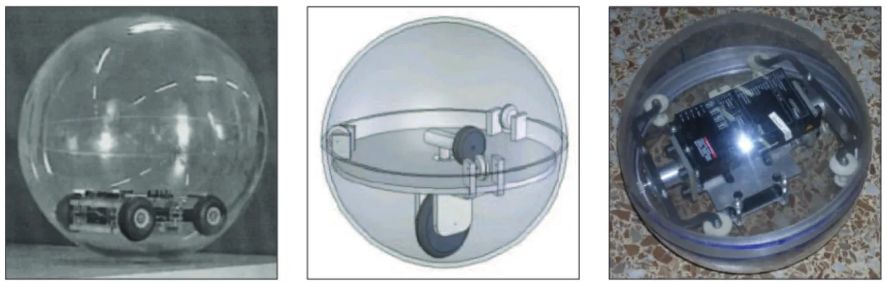
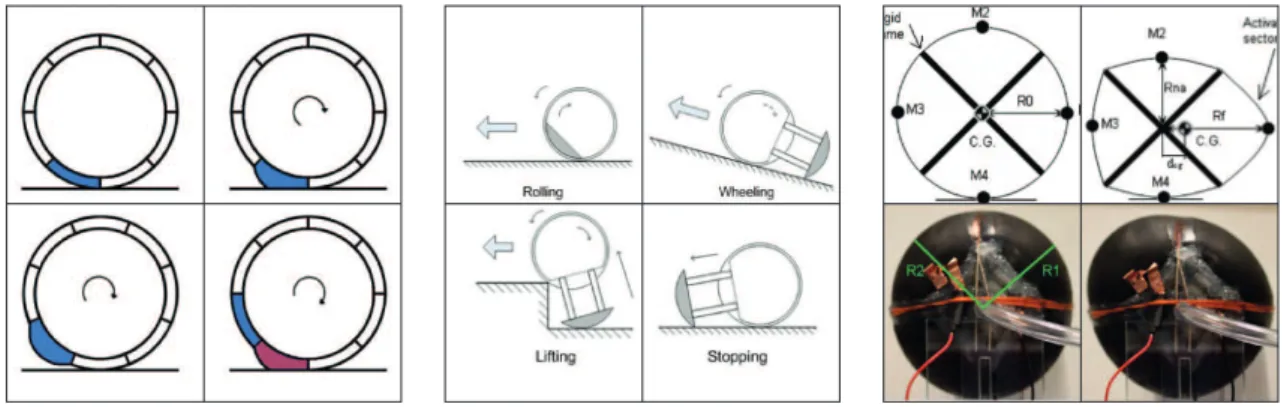
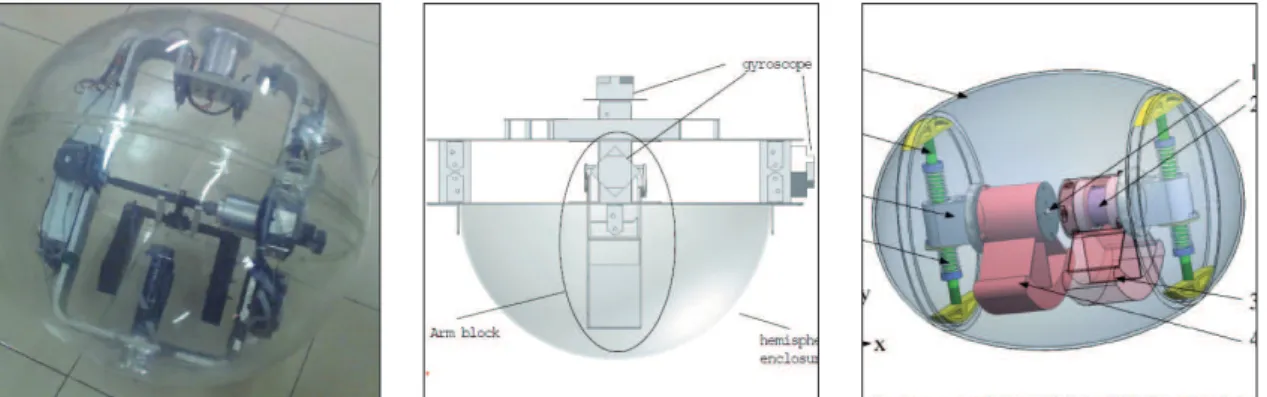
Based on the actuating schemes the spherical rolling robot can be classified into the wheel- driven type [6–8], the rotor-driven type [9–11], the pendulum-driven type [12–14] and deformable type [15–17].

For the inner wheel driven type shown in Fig. 1.1, the power that enables the robot to move is transmitted from the driving wheels to the outer shell through the friction on the contact points. However, the friction force between wheels and shell is affected dramatically under high acceleration that causes inaccuracy in control.

Figure 1.1: Inner-wheel-driven rolling robot

For spherical robot with deformable shape shown in Fig. 1.2, the motion of robot relies on transformation of its outer body. This can be achieved by deformation of the encom- passing shell, or having environmental elements, such as wind or water, act on the body itself. However due to the complexity of the driving mechanism and difficulty of modelling, accurate motion planning and control are far from completed.

For the rotor-driven type shown in Fig. 1.3, by spinning the rotors about axis fixed in the spherical shell, the laws of conservation of angular momentum can be used to control the

(14)

Figure 1.2: Deformable type rolling robot

movement of the robot. Under a proper placement of the rotors the center of mass of the composite system is at the geometric center of the sphere and, as a result, the gravity does not enter the motion equations. This facilitates the dynamic analysis and the design of the control system. However it should be noted that there exist certain types of motion that can not be realized by this driving mechanism.

Figure 1.3: Rotor-driven rolling robot

For the pendulum driven type shown in Fig. 1.4, consider the robot resting in equilibrium when pendulum is pointed to the ground. By swinging the pendulum, the mass distribution of the ball-pendulum will be shifted, causing the ball to roll to a new position of equilibrium.

With proper timing and control, the robot can move smoothly along a given path.

While the motions of spherical rolling robots appear to be aesthetically beautiful, it is far from being clear how these motions can be planned and controlled in the full state space

(15)

Figure 1.4: Pendulum-driven rolling robot

(including the orientation of the vehicle) if the dynamics of the actuators must be taken into account. Answering this question is very important for the construction of intelligent control systems for rolling robots.

1.1.2 Motion planning for underactuated systems

One of the important problems in the control of underactuated systems is the construction of motion planning algorithms. Typically, the motion planning problem requires to steer the system from an initial state to a given final state. Different from the fully-actuated systems, for underactuated systems, the underactuation feature forms a nonholonomic constraint between the configuration variables. This constraint makes the motion planning problem challenging due to that the generated motion trajectory needs to respect the constraint.

Due to the fact that underactuated systems are not invertible, like fully actuated systems, several approaches have been proposed, aiming at the approximate inversion. Such motion planning techniques include the nilpotent approximation [18], and a small amplitude and oscillatory control based method [19, 20]. Other than the approximation techniques, several directions have been explored focusing on the simplification of motion equations. In [21]

the geometric mechanics are utilized to reduce the dynamics of a system so that it can be represented as a kinematic system. In [22] the partial feedback linearization is first applied and then a concept of natural motion is utilized to generated desired motion trajectories.

Two more approaches are presented for underactuated multibody systems in [23] based on

(16)

the nonlinear coordinate transformation and the servo-constraints, respectively. Instead of approximation, other methods have been proposed for systems with special features such as the differential flatness [24, 25].

Despite the achievements, motion planning techniques proposed in the literature are usually computationally expensive and thus, cannot be run in real-time on robots. Fast approaches have rarely been explored, even for planar underactuated systems. The planar underactuated systems can be classified into two types: base-fixed type and the base-free type. The base-fixed systems are those with one or more portions of the systems fixed on the ground, such as the serial robot with passive joints. Motion planning problem for this type of systems is studied in the literature [26–30]. On the other hand, the base-free type is underactuated systems whose position and orientation can be steered freely by internal shape change. It includes the cart-pole system, the planar ballbot system [31] and the hoop- pendulum system [32]. For this type of systems, which also refers to the shape-accelerated mobile robots [31, 33, 34], very few works on the motion planning problem exist, except for the optimal control formulation which may result to heavy computational cost. In this thesis, I propose a motion planning algorithm that provides near-optimal system performance but with less computational cost. The proposed algorithm works on a class of underactuated systems that are partially differentially flat [34].

1.1.3 Control of underactuated systems

In the literature, a great number of works on the control of underactuated mechanical systems have been proposed. Among them the most popular control methods are energy shap- ing [2, 36–38], partial linearization [39–41] and sliding mode control [42–47]. A review of control methods for the underactuated mechanical systems can be seen in [48]. Despite of the accomplishment however, the control of the underactuated systems is still an active research area due to that not all underactuated systems are well controlled with the above methods. Take the instance of the nonholonomic system, a special type of underactuated system which features the nonholonomic constraints.

The proposed methods have certain requirements on some special features of mechanical systems and often are not feasible for those systems that fail to satisfy the requirements.

(17)

Instead of classifying the systems by their features and developing corresponding techniques to tackle the control problem, I intend to propose a more generic method that works on a wide class of mechanical systems. This constitutes the main goal of this research.

For control systems with equal number of inputs and states, the control matrix that weights the system inputs, is square such that a state feedback law is easily defined. How- ever in most cases, the control matrix for mechanical systems represented in the state space form, is not square due to that the number of inputs and of states are not always matched.

These systems refer to the non-square systems. In this paper, I place emphasis on a class of non-square systems where number of inputs is less than that of states.

The control problem for non-square systems is difficult because the control matrix is not invertible. The most straightforward way is to square the system by applying the pseudo inverse. However, the idea of using the pseudo inverse is to approximate the original non- square system by a square system, and the performance of this approximation requires certain properties of the pseudo inverse. These properties of the pseudo inverse for its application on the control problems of non-square system are studied by [49]. Other studies on the control problem of non-square systems either apply fuzzy control [50] or are only suitable under certain situations [51, 52]. In this paper, I propose an exact control algorithm for systems expressed by non-square state space form. The control algorithm is constructed based on the function approximation technique, inspired by its application on the adaptive control [53–56].

1.2 Major achievements

Corresponding to the three topics of my research (spherical robots, motion planning and control for underactuated systems), the major achievements can be summarized as follows.

Firstly, I proposed a motion planning and a control algorithms for spherical rolling robots.

Secondly, I extended the proposed motion planning algorithm, based on a geometric phase approach, to a class of underactuated systems, which I call the base-free systems. Thirdly, similar to motion planning, I extended the proposed control algorithm, based on the function approximation technique (FAT), to non-square systems, a broader class of underactuated

(18)

systems. In what follows, these achievements are illustrated respectively, in details.

1.2.1 Dynamic motion planning and control for a class of spherical rolling robots

A virtual constraint based decoupling algorithm was first proposed which reduced a rest- to-rest motion planning problem for ball-pendulum system to that for the hoop-pendulum system, a planar case of the ball-pendulum. The reduced planning problem could be solved through optimal control formulation seeking for minimum effort. However the optimal control based motion planning may be sensitive to the given boundary conditions and may lead to a heavy computational cost. Instead of optimal control formulation, I proposed a geometric phase based motion planning algorithm which provides similar results compared with the optimal control formulation but with less computational cost, and thus more suitable for realtime applications.

For the dynamic control problem, an adaptive trajectory tracking controller for the ball- pendulum system was constructed under a backstepping framework. The backstepping process combined two steps. A feedback velocity control input, denoted by angular velocity of the spherical shell, was first designed for the kinematic steering system. Then the specific robot dynamics were taken into account to convert a steering command into control torques acting on the pendulum. Noting that in either step, the subsystem to be controlled is underactuated, I proposed an FAT based controller and tested it under simulations. The proposed FAT based controller was proved to be adaptive to time varying uncertainties such as un-modeled system dynamics and external perturbations.

1.2.2 Geometric phase based motion planning for the base-free systems

A rest-to-rest motion planning problem was studied for a class of underactuated systems.

I first classified the planar underactuated systems into two types. One is the base-fixed systems that one or more portions of the systems are fixed on the ground, including the serial robot with passive joints. The other is the base-free type whose position and orientation can be steered freely by internal shape change, such as the cart-pole system, the ballbot system

(19)

and the hoop-pendulum system. A geometric phase based motion planning algorithm was proposed for the base-free type systems.

After the partial feedback linearization, this type of systems are commonly partially differentially flat and the base variable is the flat output. That is, the derivatives of the fiber variable of these systems can be represented purely by the base variable and its derivatives.

It leads to a property that the linearized model of these systems is then-th order integrator.

Based on this property, the motion planning algorithm has been constructed as follows.

First, the derivative of Beta-function weighted by a constant parameter was selected as a candidate for the base variable due to that it is shown to be the optimal solution for the linearized system. Its feasibility was proved by showing that the corresponding fiber variable can satisfy the given boundary conditions. Finally the parameter of the derivative of Beta-function was adjusted such that a desired shift for the fiber variable can be obtained.

Under the proposed motion planning algorithm, rest-to-rest trajectories for the configuration variables were generated with similar system performance but with less computational cost, compared with the optimal control formulation.

1.2.3 Function approximation technique based control for non-square systems

A generic control method has been proposed for the non-square systems where the number of system inputs is not equal to that of the states. Note that non-square systems are a broader class of underactuated systems. By introducing an auxiliary input the dimension of which equals that of the system state, the non-square system was restructured in the form of the combination of a square system and the variation from the original non-square system, which is treated as system uncertainties.

In the control process, the uncertainty term was replaced by its approximation as a cho- sen basis function weighted by constant parameters to be determined. These unknown plant parameters were estimated at each instant, denoted by the adjustable control parameters using a defined update law. Thus the influence to the control process caused by the variation between the auxiliary square system and the original non-square system can be eliminated.

The asymptotic stability was established for the closed loop system formulated by the

(20)

non-square system and the constructed controller. The feasibility of the proposed control method was verified under simulations for the point stabilization problem of a linear system, a nonlinear underactuated system, and a nonholonomic system, respectively.

1.3 Organization

The rest of this dissertation is organized as follows. Chapter 2 provides the motion planning and trajectory tracking control algorithms for the ball-pendulum system. Chapter 3 presents a geometric phase based motion planning algorithm for a class of underactuated systems, the base-free systems. Chapter 4 proposes a function approximation technique based control method for non-square systems. Chapter 5 provides concluding remarks and future plan.

(21)

Chapter 2 Spherical rolling robot

2.1 Background

In recent years there has been a growing interest to the study of spherical rolling robot.

Different from the vast majority of mobile robots that either have legs or exploit conventional multiple wheels, the rolling robots, considered as single wheel vehicles, represent a new type of mechanical systems demonstrating rich and intriguing dynamics. Compared with traditional mobile robots, spherical rolling robots are geometrically symmetric (cannot be turned upside down), omnidirectional and more robust (all devices are covered by a solid outer shell, including driving unit, sensors, etc.).

Encouraged by these advantages, many designs of spherical robots have been proposed.

Based on the actuating schemes the spherical rolling robot can be classified into the wheel- driven type [6–8], the rotor-driven type [9–11], the pendulum-driven type [12–14] and deformable type [15–17]. My work is related to the pendulum-driven type. We study a class of spherical rolling robots driven by a 2DOF pendulum, which we call the ball-pendulum systems. The ball-pendulum system is selected due to the following reasons. Firstly, the driven mechanism is simple. Secondly, this type of diving mechanism can realize motion of the sphere along any shape of smooth contact curves. Thirdly, the control for this type of spherical robot is still an open problem.

One of the important research problems for control of mobile robot is to steer the robot

(22)

from an initial configuration to the final configuration. For the spherical rolling robot we need not only to steer the position of the sphere but also the orientation of the sphere. The control for the orientation is important when it is necessary to attach some devices such as sensors or camera in or out of the shell, or when it is required to know where the robot is heading. The steering problem seems to be a normal point to point stabilization problem which can be solved by constructing a continuous feedback. However, spherical rolling robots are special because it is a nonholonomic system. According to the Brockett theory [57], there exists no continuous feedback for local asymptotic stabilization of an equilibrium point. Instead of apply direct feedback methods, we plan to solve the steering problem step by step.

The main process is as followed. One can first design a path on the ground, connecting the start and the goal configurations of the spherical shell, by using conventional kinematic planners [71–75]. With a given feasible path, one can plan the motion trajectories for both the orientation and the position of the sphere when it is tracing this path. This step is called motion planning. In the real application however, the actual motion of the ball-pendulum system may deviate from the desired trajectory due to unexpected disturbances such as the friction or uneven terrain. To deal with this problem, one needs to construct a feedback control law such that the actual motion of the spherical rolling robot will converge to the desired. We call this step the trajectory tracking. Through these two steps, one can steer the ball-pendulum system from initial to final configurations in a rest-to-rest mode even under perturbations.

The rest of this chapter is organized as follows. In Section 2.2, one provides the contact kinematics and dynamic model for the ball-pendulum system. In Section 2.3, a motion planning algorithm is proposed that enables the spherical robot to trace given contact path on the ground in a rest-to-rest mode. In Section 2.4, a feedback control method is developed such that the actual motion trajectory of the ball-pendulum system can converge to the trajectory designed in Section 2.3 under perturbation. Finally, a summary is given in Section 2.5.

(23)

2.2 Mathematical Model

X

Y Z

q₁ q₂

Σo

Σb

(uo, vo) c

(ub, v_b) c

ψ Σcb

Σco

Figure 2.1: Ball-pendulum system formalization.

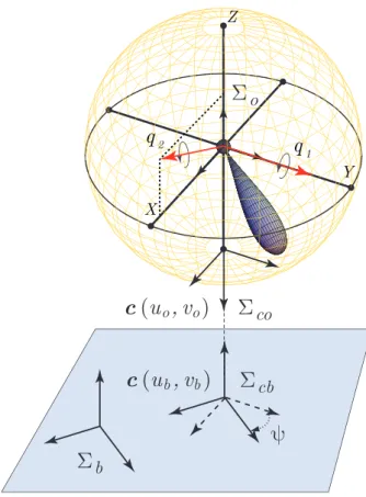
Consider a rolling robot composed of a homogenous spherical shell actuated by a pendulum. It is assumed that the pendulum is mounted at the geometric center of the shell as shown in Fig. 2.1 and is actuated by two motors.

To describe the contact kinematics, we introduce the following coordinate frames: Σois a frame fixed at the geometric center of the sphere,Σ_b is a frame fixed at the contact plane.

In addition, at the contact point we introduce the contact frame of the object Σ_co, and the contact frame of the plane,Σ_cb, which is parallel toΣ_b.

The contact coordinates are given by the anglesu_o andv_o, describing the contact point on the sphere, andu_b andv_b, describing the contact point on the plane, and by the contact angleψ which is defined as the angle between thex-axis ofΣcoandΣcb

(24)

2.2.1 Contact Kinematics

The position of the contact point on the sphere, denoted by the vector ρ_cand expressed in the axis ofΣ_o, is parameterized as

oρ_c=R_y(u_o)R_x(v_o)





 0 0

−R







=R







−sinu_ocosv_o sinv_o

−cosuocosvo







, (2.1)

whereRis the radius of the sphere. In this parameterization the origin is placed at the south pole of the sphere. The parameterization defines the Gaussian frameΣ_co whose orientation relative toΣ_ois given by the matrix^oR_co(u_o, v_o) =R_y(u_o)R_x(v_o)R_y(π), composed of the elementary rotations. Note that instead of the classical Euler angles and their variations we define the orientation of the sphere in terms of the contact coordinatesu_o, v_o andψ.

Let ωo = (ωx, ωy, ωz) be the angular velocity of the frame Σo, defined in projections onto the axis of the base frameΣ_b. The evolution of the contact coordinates is described by Montana’s equations [58], which in our parameterization take the following form







˙ u_b

˙ v_b

˙ u_o

˙ v_o ψ˙







=







0 R 0

−R 0 0

−sinψ/cosv_o −cosψ/cosv_o 0

−cosψ sinψ 0

−sinψtanvo −cosψtanvo −1











 ω_x ω_y ω_z







. (2.2)

2.2.2 Dynamic Model

In what follows, the derivation of the dynamic models will be conducted with the use of D’Alembert’s principle. Letrobe the vector of the origin of the frameΣo(see Fig. 2.2),vo

its absolute velocity, andω_o the angular velocity of the frameΣ_o. The virtual displacement of the origin of Σ_o is denoted by δr_o, and the vector of infinitesimal rotation of Σ_o with

(25)

ρ

c

r

c

r

o

Σ

o

Σ

b

r

p

ρ

p

Σ

p

Figure 2.2: Definition of basic vectors.

respectΣ_bis denoted byδπ_o. Unless otherwise specified all the vector and tensor quantities are assumed to be expressed in the axes of the inertial frameΣ_b.

The frameΣ_p is attached to the pendulum and its origin coincides with that ofΣ_o. Let ρ_p be the vector of the center of mass of the pendulum with respect to the frameΣo, vp its absolute velocity, andω_relthe angular velocity of the frameΣ_pwith respect toΣ_o. The vector for the infinitesimal rotation ofΣ_p with respect toΣ_ois denoted byδπ_rel. The kinematics of the pendulum are defined by the following relationships

δπp = δπo+δπ_rel, (2.3)

ω_p = ω_o+ω_rel, (2.4)

˙

ω_p = ω˙_o+ω_o×ω_rel+ ˙ω_rel, (2.5)

vp = vo+ωp×ρ_p, (2.6)

˙

v_p = v˙_o+ ˙ω_p×ρ_p+ω_p×(ω_p×ρ_p). (2.7) For system under consideration free from the rolling constraint D’Alembert’s principle can be written down as follows [59]

δr_o·

m_o( ˙v_o−g)+m_p( ˙v_p−g)

+δπ_o·

J_oω˙_o+ω_o×J_oω_o +δπ_p·

m_pρ_p×( ˙v_o−g)+J_pω˙_p+ω_p×J_pω_p

=δW, (2.8) where g is the gravity vector, m is the mass of the spherical shell, and Jo = ²₃mR²I its

(26)

inertia tensor with respect to the origin of Σo, mp is the mass of the pendulum, and Jp

is the inertia tensor of the pendulum with respect to the origin of Σ_p. The virtual work δW =δπ_rel·M, whereM is the moment generated by the actuators.

The derivation of dynamic equations is conducted in several steps by transforming (2.8) to independent variations. First, we transform the virtual displacement δr_o in (2.8) to the point of contact, defined by the vectorr_c. The reason is to introduce variations of quasi- coordinates that would vanish by virtue of the non-holonomic constraints [60, 61]. Note that r_c=r_o+ρ_c and thereforeδr_c=δr_o+δπ_o×ρ_c, whereρ_c is the vector emanated from the center of mass of the sphere to the contact point. The rolling constraints, formulated in terms of the variations of the quasi-coordinates, can be written down asδr_c= 0, and therefore

δro=−δπo×ρ_c. (2.9)

Upon substituting (2.9) into (2.8) and transformingδπ_p toδπ_o andδπ_relby using (2.3), one obtains

δπ_o·

J_oω˙_o+J_pω˙_p+ω_p×J_pω_p−ρ_c×(mv˙_o+m_pv˙_p)+m_pρ_p ×( ˙v_o−g) + δπ_rel·

m_pρ_p×( ˙v_o−g) +J_pω˙_p+ω_p×J_pω_p−M

=0. (2.10)

Next, we take into account the rolling constraint v_o +ω_o×ρ_c = 0 and establish the velocity and acceleration of the spherical shell:

v_o =−ω_o×ρ_c, v˙_o =−ω˙_o×ρ_c. (2.11) By expressing vp andv˙p in (2.6, 2.7) through, respectively,ωo, ω_rel, andω˙o, ω˙_rel with the use of (2.4, 2.5) and (2.11), one converts (2.10) to the following form

δπ_o·

H_ooω˙_o+H_opω˙_rel+h_o

+δπ_rel·

H_poω˙_o+H_ppω˙_rel+h_p−M

= 0, (2.12)

(27)

where

H_oo = J_c+J_p+m_p(ˆρ_pρˆ_c+ ˆρ_cρˆ_p), H_op=J_p+m_pρˆ_cρˆ_p, H_po=H^>_po, H_pp =J_p, h_o = ω_p ×J_pω_p−m_p ρ_p×g+ρ_c×(ω_p×(ω_p×ρ_p))

, h_p = ω_p ×J_pω_p−ρ_p×m_pg.

Here in the equations, J_c = J_o−(m+m_p)ˆρ_cρˆ_c is the inertia tensor of the rolling robot with respect to the contact point, and by hat we denote the skew-symmetric operator such thata×b≡ab.ˆ

Note that variationδπ_relis not independent as the pendulum is assumed to be driven by two actuators. The relative position of the pendulum with respect toΣo can be described by two angles,q₁ andq₂, mimicing the contact coordinatesu_oandv_o. Under this definition, the pendulum is rotated along the axes defined (in the frameΣ_o) by the unit vectorse₁ = (0,1,0)ande₂ = (cosq₁,0,−sinq₁), and the orientation ofΣ_pwith respect toΣ_ois defined by the matrix^oR_p =R_y(q₁)R_x(q₂).

Letq = (q₁, q₂)be the vector of the generalized coordinates of the pendulum andτ = (τ1, τ2)the vector of the driving torques. The relative kinematic quantities and the moment generated by the actuators are defined as

δπ_rel=Eδq, ω_rel=Eq,˙ ω˙_rel=E¨q+e, M =Eτ, (2.13) whereE= [e₁|e₂], ande= (e₁×e₂) ˙q₁q˙₂. Now, by plugging (2.13) into (2.12) and treating δπ_o andδqas the independent variations, one finally obtains the dynamic equations for the rolling carrier and the pendulum:







H_oo H_op H_po H_pp













˙ ω_o

¨ q





+





 h_o h_p





=





 0 τ





, (2.14)

(28)

where

H_oo = H_oo,H_op =H_opE,H_po=H^>_op,H_pp =E^>J_pE, h_o = h_o+H_ope,h_p =h_p+E^>H_ppe.

Note that the number of equations in the dynamic model (2.14) is minimal since the reaction forces associated with the rolling constraint have been eliminated by reducing the motion equations to the independent variations. By converting the dynamic equations (2.14) to the 1st order form and combining them with the kinematic equations (2.2), one obtains the state space modelx˙ =f(x,u), with 12-dimensional state vectorx= (u_b, v_b, u_o, v_o, ψ, ω_x, ω_y, ω_z, q₁, q₂,q˙₁,q˙₂)and 2-dimensional control inputu=τ.

(29)

2.3 Motion Planning

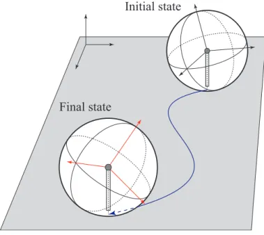
Initial state

Final state

Figure 2.3: Motion planning problem.

One of the important problems in the control of spherical rolling robots is the construction of motion planning algorithms for steering the robot from an initial configuration of the spherical shell, defined by its position and orientation, to a final one. Typically, the steering is organized in the rest-to-rest mode. In literature, this motion planning problem is considered mostly for a ball-plate system, with the ball driven externally by two parallel plates, and solved in kinematic formulation [71–75]. For the rolling robots actuated by internal motors, the control system based on the kinematic planner can operate in the quasi-static mode [10, 65, 76, 77], presuming relatively slow movements.

To realize faster and more accurate movements for the ball-pendulum system, it is necessary to extend the motion planning algorithms from the kinematic to dynamic domain. A generic way is to plan motion based on the full model which takes into account both the kinematics and dynamics of the robot. The full model is described by twelve states and two control inputs. It is highly nonlinear and features both the non-holonomic rolling constraint and the gravitational drift term. As a result, only generic techniques such as optimal control

(30)

can be employed for solving the motion planning problem. However, they come with a high computational cost.

To avoid the difficulties of motion planning based on the full model, one can try to decouple the problem into kinematic and dynamic stages and solve them separately. Specif- ically, one can first design a feasible path, connecting the start and the goal configurations of the spherical shell, by using conventional kinematic planners [71–75]. Then, one can try to generate timing control laws, based on the dynamic model of the spherical shell and the actuators, tracing the feasible path in rest-to-rest mode. However, the decoupling approach does not necessarily work for all types of rolling robots and it depends on the type of ac- tuation. For instance, it was shown that for rolling robots actuated by two rotors not any kinematically feasible motion is dynamically realizable [78].

It should be noted that motion control in dynamic formulation was addressed in [7, 79–

82]. In [79, 82], only partial cases (rolling along a straight line or a circle) were considered.

In [7, 80], the motion of the spherical robot along complex curves was decomposed into forwarding and turning. However, this decomposition is not accurate because the effect of the dynamic interaction between these two basic movements was neglected in the dynamic model. Similarly, a simplified decoupled model, ignoring dynamic interaction between rotation of the sphere along the transversal and longitudinal directions, was used in [81].

In Section 2.3.1, we show that any feasible kinematic motion of the sphere, considered in the class of pure rolling (no spinning) motion, is dynamically realizable in the ball-pendulum system. As a result, the motion planning problem can be decomposed into kinematic and dynamic stages. Moreover, by introducing a virtual constraint corresponding to pure rolling mode, the dynamic model is reduced to just two equations describing motion of an underactuated hoop-pendulum system along the contact path. We show that the hoop-pendulum system is controllable and this implies the controllability of the ball-pendulum system since the sphere rolling without spinning is controllable [71]. Next, we show that the form of the dynamic equations of the hoop-pendulum system is invariant with respect to the feasible contact path. This implies that a wide variety of kinematically feasible motions (pure rolling movements) can be dynamically realized by a single underactuated system. To plan rest-to-rest movements of the hoop-pendulum system, we use a geometric phase approach

(31)

and show its connection to and comparison with the optimal control problem where the minimum control effort is taken as the performance index.

Motion planning for the ball-pendulum system requires to steer the spherical robot from an initial configuration to a final configuration. The problem can be stated as finding a trajectoryx(t), t ∈ [0, T], given the start statex(0) = x_s and the final state x(T) = x_f. It is assumed that the system is at rest at the start and final configurations, i.e. ω_o(0) = ωo(T) = 0, q(0) = ˙˙ q(T) = 0. Also, since the pendulum at the rest configurations is pointed downward, we have q₁(0) = u_o(0) = 0, q₁(T) = u_o(T) = 0,q₂(0) = v_o(0) = 0, q₂(T) = v_o(T) = 0. This reconfiguration problem is illustrated in Fig. 2.3.

Note that the kinematic (2.2) and dynamic (2.14) models are coupled through the angular velocity of the spherical shell ω_o(t). Also note that the twelve-dimensional state space model, obtained from (2.2,2.14), is a nonlinear control-affine system with the drift term and two control inputs. Motion planning for such a system in the general settings can be cumbersome and require the use of generic techniques such as optimal control.

2.3.1 Dynamic realizability

An alternative approach to the motion planning problem would be to decompose it and solve it separately at the kinematic and dynamic levels. At the kinematic level, one constructs a feasible path and findωo(t)based on the kinematic model (2.2). At the dynamic level, one finds the trajectory of the pendulum and establishes the timing control law for the actuators tracing the kinematically feasible path.

However this decoupling approach does not always work since not any angular velocity of the spherical shall ω_o(t)is dynamically realizable. The planned trajectory for unrealiz- ableω_o(t)is invalid due to that physically unrealizable motions cannot be generated by the driving mechanisms. As far as we know, the dynamic realizability for the ball-pendulum system has not been addressed in the motion planning literature. In this chapter, we first define the dynamical realizability condition mathematically. Then, we propose a dynamically realizable decoupling technique such that the motion planning problem can be decomposed into kinematic and dynamic stages, and thus solved separately. This is the novelty of our work in the motion planning for the ball-pendulum system.

(32)

Referring to the dynamic model for the ball-pendulum system (2.14), if hn is a vector parameterizing the null space of matrixH_po, one has

h_n·(H_ooω˙_o+h_o) = 0, (2.15) which can be called the condition of dynamic realizability. Hence, the kinematical motion of the sphere, represented by ω_o(t) can be accomplished by the actuators only when the dynamic realizability condition is satisfied.

A notable unrealizable case is when the ball-pendulum system is at rest: (ω_o,q,q) =˙ 0, where the dynamic realizability condition (2.15) does not hold true unless the magnitude of the angular acceleration of the sphere kω˙ok or itsz-axis component ω˙z equals to zero.

This can be proved by the substitution of(ω_o,q,q) =˙ 0into (2.15), where the corresponding h_n = (0,0,1). Through simple calculations, one can show that the left hand side of (2.15) equals to zero only whenkω˙_ok = 0orω˙_z = 0. For instance, a straight line motion of the sphere, expressed byω_o = ^√¹

3(1,1,1) sin(t), is not realizable by the 2DOF pendulum in rest-to-rest mode, due to that at a rest configuration, the condition of the dynamic realizability (2.15) is not satisfied.

Noting that instantaneous spinningω_zmay lead to unrealizable motions of the spherical carrier, we adopt only pure rolling (ω_z = 0) in our motion planning algorithm. In what follows, we show that a class of motions corresponding to pure rolling of the carrier, actuated by a two DOF pendulum, is dynamically realizable. To show the realizability, instead of checking the null space of matrixH_po, we develop a dynamic model of the ball-pendulum system, reduced by the pure rolling constraint and establish its controllability. The reduced dynamic model is an underactuated system, a hoop-pendulum system, described by two differential equations with single control input. It is invariant to the shape of the contact path, and the dynamic motion planner can be constructed in a unified manner.

As a result, motion planning for the ball-pendulum system can be decoupled into kinematic and dynamic levels. In the kinematic level, one designs a path on the contact plane connecting the start and the goal points, such that if the sphere rolls along this path, it can reach the goal with a desired orientation. In the dynamic level, one constructs torques on the pendulum, the actuator, to generate the time trajectories for the rolling motion of the

(33)

ball-pendulum system along the designed path. The kinematic problem can be solved by planners available in the literature [71–75], while the dynamic problem is tackled with a decoupling based algorithm we developed, the details of which are demonstrated in the following sections.

2.3.2 Virtual constraint based reduction of dynamic model

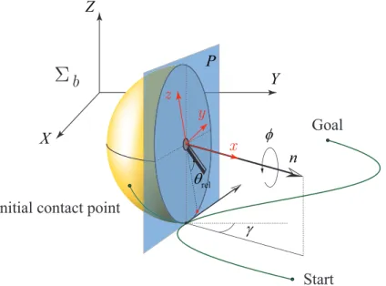
Start Goal

Initial contact point

Y Z

X

P

n x f

y z

qrel

g

Σ

b

Figure 2.4: Spherical robot tracing given contact path.

Assume the spherical shell rolls without spinning along a path constructed by the kinematic planner as shown in Fig. 2.4. Let φ be the angular distance of the center of the sphere such that the current length of the contact path on the plane is 2πφ. Let also n = (sinγ,cosγ,0) be the vector normal to the contact path on the plane, where γ is the angle between vectorn and the Y-axis of the coordinate frameΣ_b. Since the angular velocity of the sphere under rolling without spinning does not havez-component, the virtual constraint corresponding to pure rolling can be formalized as

δπ_o =nδφ, ω_o =nφ,˙ ω˙_o =nφ¨+ ˙nφ.˙ (2.16)

(34)

Let P be the vertical plane instantaneously tangent to (moving along) the contact path as shown in Fig. 2.4. To realize the pure rolling motion of the sphere, the center of mass of the pendulum must (instantaneously) move in the planeP. If the pendulum is axisymmetric with respect to the line through its center of mass, the angular velocity of the pendulum must be directed along the normal vector n. Letθ_rel be the angle of rotation of the pendulum in the planeP through the normal vectorn. The virtual constraint imposed on the motion of the pendulum can be formalized as

δπ_rel =nδθ_rel, ω_rel =nθ˙_rel, ω˙_rel=nθ¨_rel+ ˙nθ˙_rel. (2.17) By plugging the virtual constraints (2.16, 2.17) into (2.12) and treating δφandδθ_rel as the independent variations, one obtains two equations describing the reduced dynamics:

n^>H_oon φ¨+

n^>H_opn

θ¨_rel+n^>

H_oon˙φ˙ +H_opn˙θ˙_rel+h_o

= 0, (2.18)

n^>H_pon φ¨+

n^>H_ppn

θ¨_rel+n^>

H_pon˙φ˙+H_ppn˙θ˙_rel+h_p

=τ_θ,(2.19) where τ_θ = n^>M represents the control torque reduced to the coordinate θ. It is the projection of the momentM =Eτ generated by the control torquesτ onto the line through the vectorn.

Note that equation (2.18) describes motion of the rolling carrier along the given contact path, which can be called a virtual hoop, while equation (2.19) does the motion of the pendulum in the moving plane P. To distinguish the reduced dynamic system from the main one, we call it the hoop-pendulum system and illustrate it by Fig. 2.5. The red dot on the hoop is its initial contact point to the ground. One revolution of the initial contact point implies a2πRlinear displacement for the center of the hoop. Note that at the starting configuration (φ(0) = 0), the initial contact point touches the ground.

As shown in Appendix A, the calculation of terms in (2.18, 2.19) under the assumption that the pendulum is a beam with uniform mass distribution yields the following represen-

(35)

q 2l z

y

tq

f

qrel

P

So

Figure 2.5: Hoop-pendulum system.

tation

J_c+J_p−2m_pRlcos(φ+θ_rel) φ¨+

J_p−m_pRlcos(φ+θ_rel) θ¨_rel +mplsin(φ+θ_rel)

R( ˙φ+ ˙θ_rel)²+g

= 0, (2.20)

J_p−m_pRlcos(φ+θ_rel)

φ¨+J_pθ¨_rel+m_pglsin(φ+θ_rel) =τ_θ, (2.21) with J_c = J_o+ (m+m_p)R² where J_o is inertia moment of the hoop with respect to the center of the hoop,J_pis the inertia moment of the pendulum with respect to the center of the hoop, lis the half-length of the projection of the pendulum onto the planeP, andg stands for the gravitational acceleration.

To represent the hoop-pendulum dynamics in a more compact form, one can introduce the angleθ =θ_rel+φ, defining the orientation of the pendulum with respect to the ground.

Upon transformation of motion equations (2.20, 2.21) fromθ_reltoθ, one obtains

J_c−m_pRlcosθ φ¨+

J_p−m_pRlcosθ

θ¨+m_plsinθ

Rθ˙²+g

= 0, (2.22)

−m_pRlcosθφ¨+J_pθ¨+m_pglsinθ = τ_θ. (2.23) Three important remarks are in order.

1. Motion equations (2.22, 2.23) have already been derived in the literature (see [83, 84]

and references therein) for the case of rolling along a straight line, which is a partial

(36)

case of pure rolling. Our derivation shows that the form (2.22, 2.23) holds true for any contact path compatible with the assumption of pure rolling.

2. Any motion of the sphere along the contact path is dynamically realizable by the pendulum (if the actuators are powerful enough), as for any φ(t) one can always find θ(t)by solving differential equation (2.22). Therefore, motion planning for the ball- pendulum system can be, in principle, decomposed to the kinematic (ball-plate system) and dynamic (hoop-pendulum system) levels.

3. Motion equations (2.22, 2.23) do not feature the angleγ defining the orientation of vectorn. Thus, the form (2.22, 2.23) is invariant to the shape of the contact curve.

As a result, motion planning for the hoop-pendulum system covers a large variety of contact paths corresponding to pure rolling in a unified way.

2.3.3 Motion planning for the reduced system

The hoop-pendulum is an underactuated system where (2.22) forms a second order nonholonomic constraint. In planning the rest-to-rest movements for such a system, it is always an option to make use of a generic optimal control formulation with different performance indices. However, it comes with a higher computational cost. Instead, we employ the geometric phase approach to motion planning of underactuated systems [1] in which generation of closed-loop trajectories for base variables results in the propulsion of the fiber variables.

Note from the nonholonomic constraint (2.22) that φ¨can be expressed by only θ and its derivatives. Therefore, the hoop angleφand the pendulum angle θare treated respectively as the fiber and base variables.

By solving (2.22) for φ¨ and plugging it in (2.23), one establishes the static feedback control law

τ_θ =

J_p+m_pRlcosθ(J_p −m_pRlcosθ) J_c−m_pRlcosθ

u

+mplsinθ g+m_pRlcosθ(g+Rθ˙²) J_c−m_pRlcosθ

!

, (2.24)

(37)

transforming the hoop-pendulum dynamic equations (2.22, 2.23) to the following represen- tation

φ¨ = −m_plsinθ(g+Rθ˙²) + (J_p−m_pRlcosθ)u

J_c−m_pRlcosθ , (2.25)

θ¨ = u, (2.26)

whereuis treated as a new control input. In the state-space form

˙ x_hp =







φ˙

−^m_J^p^l^sin^θ(g+R^θ^˙²⁾

c−mpRlcosθ

θ˙ 0





 +







0

−^J_J^p^−m^p^Rl^cos^θ

c−mpRlcosθ

0 1







u, (2.27)

wherex_hp = (φ,φ, θ,˙ θ). Note that the collocated feedback linearization (2.24) is defined˙ globally sinceJ_c > m_pRl.

Consider first small motion of the hoop-pendulum system around an equilibrium config- urationx_hp(0)orx_hp(T)where

x_hp(0) =0, x_hp(T) = (φ_des,0,0,0). (2.28) The linearization of (2.27) atx_hp(0)orx_hp(T)is defined as

x˙_hp =Ax_hp+bu, (2.29)

where

A=







0 1 0 0 0 0 a 0 0 0 0 1 0 0 0 0





 , b=





 0 b 0 1





 ,

(38)

with

a =− mpgl

J_c−m_pRl, b=−Jp−mpRl J_c−m_pRl.

Note that the linearized system (2.29) is controllable, which implies that the original nonlinear system (2.27) is locally controllable around the equilibrium.

Under the dynamic constraints (2.29) and the boundary conditions (2.28), the optimal solution, minimizing the control effort

J = 1 2

Z T 0

u²(t)dt, (2.30)

is defined as [85]

x_hp(t) = e^AtW(t)W(T)⁻¹e^−ATx_hp(T), (2.31) where

W(t) = Z t

0

e^−Asbb^>e^−A^>^sds. (2.32) It can be shown that the optimal trajectories of the hoop and the pendulum, calculated by (2.31), are expressed through the symmetric regularized incomplete Beta-function of 4-th order and its second derivative:

φ(t) = B(4,4, t/T)φ_des+ b a

B(4,¨ 4, t/T)φ_des, (2.33) θ(t) = 1

aB(4,¨ 4, t/T)φ_des, (2.34)

where

B(4,4, t/T) = t⁴(20t³−70t²T + 84tT²−35T³)

T⁷ , (2.35)

B(4,¨ 4, t/T) = 420t²(t−T)²(T −2t)

T⁷ . (2.36)

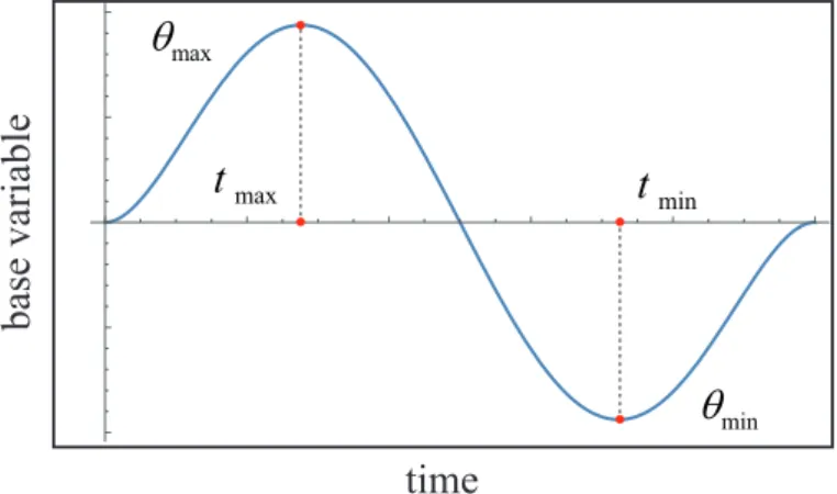
A profile of the shape variable θ(t) is shown by Fig. 2.6. It is an odd function with respect to the middle point t = T /2, with the extremal points θ_min and θ_max = −θ_min