中性子寿命測定の高精度化に関する研究

(1)

九州大学学術情報リポジトリ

Kyushu University Institutional Repository

中性子寿命測定の高精度化に関する研究

富田, 龍彦

http://hdl.handle.net/2324/1959072

出版情報：Kyushu University, 2018, 博士（理学）, 課程博士バージョン：

権利関係：

(2)

Studies on improvement of neutron lifetime measurement

–中性子寿命測定の高精度化に関する研究 –

九州大学大学院理学府物理学専攻粒子物理学分野素粒子実験研究室

富田龍彦

指導教員川越清以 September 2, 2018

(3)

(4)

Abstract

The neutron lifetime (τ_n) is one of the most important parameters in Big-Bang Nucle- osynthesis (BBN) and the Cabibbo–Kobayashi–Maskawa (CKM) matrix. Currently, τ_n = 880.2 ±1.0 sec is determined with two major methods. One of them is called the proton counting method. In this method, τ_n is determined by the neutron flux and the number of protons from β decay. Its precision is limited by uncertainty in the eﬃciency correction because these two values are determined in diﬀerent detectors. The other method is the storage method using Ultra Cold Neutrons (UCNs). This method uses a material bottle to trap UCNs.

τ_ncan be calculated with the ratio of the introduced neutrons to surviving neutrons. However, the interaction between the neutrons and the wall of the bottle introduces considerable uncertainties. While these two methods can both determine τ_n (proton counting: 888.0±2.0 sec, UCN storage: 878.6±0.6 sec), there is a 3.9 σ (8.4±2.2 sec) discrepancy. In order to verify this discrepancy, we are developing a third method at the Japan Proton Accelerator Research Complex (J-PARC). This method is based on the electron counting method which was origi- nally established by Kossakowski et al. in 1989. In this method, we count electrons generated by neutron β decay using a Time Projection Chamber (TPC) at 100 kPa. We can count not only electrons, but also the neutron flux simultaneously with the same detector. As a result, it is possible to eliminate the uncertainties that have been problematic with the existing two methods. The final goal of our experiment is 0.1% accuracy. From data acquired until 2016, we obtained a first physical result of τ_n = 896±10(stat.) ⁺¹⁴₋₁₀(sys.) sec. Through this analysis, it was found that the background caused by neutron which is scattered by operating gasses is a considerable uncertainty factor.

In this thesis, we describe an attempt to reduce the background events caused by scattered neutrons by reducing the operating gas pressure. The purpose of this attempt is to suppress the scattered neutrons by reducing the the number of operating gas nuclei. We also aim to confirm the robustness of our experiment under low operating gas pressures. We tested our TPC with a pressure of lower than 50 kPa in 2016. From this test, it was found that the heat generation in the amplifier and decrease in detection eﬃciency due to the decrease in wire gain are important problems to solve. Therefore, we developed a low heat generation amplifier by using an Application Specific Integrated Circuit (ASIC) and its read out system, and we evaluated the basic characteristics of this amplifier. As a result of this evaluation, we confirmed that the new amplifier can reduce the heat generation by a factor of 50 compared to the amplifier that we currently use. Through this development, we expect feasible low gas pressure operation from the viewpoint of hardware requirements. Therefore, in November 2017, we carried out a physics run with a gas pressure of 50 kPa. Data collection was carried out over a week, and we obtained data with 1.8% statistical accuracy. For the analysis of this data, we constructed a Monte Carlo simulation at 50 kPa, optimized the method of event selection, and estimated the various uncertainties. Finally, we obtained the result ofτ_n = 917±16(stat.)±19(sys.) sec.

This result is consistent with the measurement at 100 kPa within the uncertainties.

From the results of this study, we can solve the issue of heat generation by using the newly developed amplifier. Thus, we can carry out the experiment with much lower gas pressures to reduce the number of background events caused by scattered neutrons. We also obtained a result that is consistent with 100 kPa even at 50 kPa. This shows that our experimental apparatus and analysis method are robust to changes in the gas pressure, and we can expect to improve our experimental accuracy with the lower gas pressures operation in the future.

(5)

(6)

List of Figures

1.1 Feynman diagram of neutron beta decay. . . 12

1.2 Relationship among neutron wavelength, velocity, and energy. . . 13

1.3 Relationship among CKM unitarity, V_ud and λ. . . . 15

1.4 History of neutron lifetime measurements. . . 16

1.5 Neutron lifetime measured by the proton counting method and UCN storage method. . . 16

1.6 Schematic view of the proton counting method at the NIST. . . 17

1.7 Schematic view of the experimental apparatus at the ILL in 2005. . . 19

1.8 Schematic view of the experiment at Los Alamos. . . 20

1.9 Arrangement of the Halbach array. . . 20

1.10 Schematic view of Kossakowski’s experiment. . . 21

2.1 Conceptual diagram of the gas introduction. . . 24

2.2 Aerial photograph of J-PARC. . . 25

2.3 Schematic top-view of the MLF . . . 27

2.4 Neutron source at the MLF . . . 28

2.5 Schematic view of BL05 . . . 29

2.6 Setup for neutron lifetime measurement at J-PARC. . . 30

2.7 Schematic top-view (top) and the photograph (bottom) of the SFC . . . 31

2.8 Time structure of the MLF beam and bunch structure of BL05. . . 32

2.9 Picture of the beam monitor. . . 33

2.10 Picture of the ⁶LiF shutter. . . 33

2.11 Photograph of the TPC . . . 34

2.12 Inside photograph of the TPC. . . 35

2.13 Alignment of each wire of the MWPC. . . 36

2.14 Block diagram of the data acquisition system. . . 37

2.15 Snapshot of the simulated apparatus in the simulation. . . 39

2.16 Summary of neutron lifetimes for all three methods. . . 40

3.1 Illustration of a background event caused by a scattered neutron. . . 44

3.2 Gain at 100 kPa. . . 46

3.3 Gain at 25 kPa. . . 47

3.4 Temperature during low gas pressure operation. . . 48

3.5 Simplified block diagram of the GTARN amplifier. . . 50

3.6 Photograph of the GTARN amplifier. . . 50

3.7 Photograph of the additional amplifier. . . 51

3.8 Photograph of the module for the developed amplifier. . . 52

(9)

8 LIST OF FIGURES

3.9 Schematic diagram of the measurement for gain evaluation. . . 53

3.10 Gain linearity of the GTARN amplifier. . . 54

4.1 Distribution of the FCE. . . 59

4.2 Schematic view of “beam on” and “beam oﬀ” setups. . . 61

4.3 Distribution of the TOF. . . 62

4.4 Conceptual view for determining the fiducial region. . . 63

4.5 Two-dimensional distribution of the TOF and cathode hit information. . . 64

4.6 TOF distribution with superimposed the fiducial and sideband regions. . . 65

4.7 Example of drift lengths of the cosmic ray background and aβ decay signal. . . 66

4.8 Distribution of the drift length. . . 67

4.9 Conceptual picture of the DC. . . 68

4.10 Distribution of the DC. . . 69

4.11 Distribution of the deposit energy in the TPC. . . 70

4.12 Conceptual picture of the x-value. . . . 71

4.13 Distribution of x-values. . . . 72

4.14 Distribution of the deposit energy onto the field wire. . . 74

4.15 Photograph of the mass spectrometer. . . 76

4.16 Distribution of the deposit energy in the low voltage operation. . . 80

4.17 Summary of neutron lifetimes from all three methods. . . 84

A.1 Circuit of GTARN amplifier. . . 88

A.2 Board layout with three GTARN amplifiers. . . 89

A.3 Board layout of additional amplifier. . . 90

A.4 Circuit of additional amplifier. . . 91

A.5 Board layout of read out module. . . 92

A.6 Circuit of read out module. . . 93

(10)

List of Tables

1.1 Basic properties of the neutron. . . 12

2.1 Basic specifications of J-PARC. . . 25

2.2 Specifications of BL05 . . . 29

2.3 Specifications of the TPC . . . 35

2.4 List of Monte Carlo samples. . . 38

3.1 Scattering and absorption cross sections of various nuclei for 2200 m/s neutrons. 43 3.2 Voltage applied to the anode wire for each gas pressure. . . 45

3.3 Specifications of the newly developed amplifier. . . 55

4.1 Data acquisition sequence. . . 57

4.2 DAQ cycle in low voltage operation. . . 58

4.3 Number of background events estimated by Monte Carlo simulations. . . 73

4.4 Numbers of signal candidates. . . 73

4.5 Eﬃciencies for neutron β decay for each cut. . . 75

4.6 Eﬃciencies for neutron absorption by³He. . . 75

4.7 Contamination of¹⁴N and ¹⁷O. . . 79

4.8 Uncertainties in the cut eﬃciencies for neutronβ decay candidates. . . 80

4.9 Uncertainty in the cut eﬃciency for neutron absorption by³He candidates. . . . 81

4.10 Summary of uncertainties. . . 81

4.11 Corrections and uncertainties for each analysis procedure for β decay events. . . 82

4.12 Corrections and uncertainties for each analysis procedure for ³He events. . . 82

4.13 Summary of the analysis. . . 83

(11)

(12)

Chapter 1 Introduction

1.1 Overview of this thesis

This thesis describes studies for improving neutron lifetime measurements at the Japan Proton Accelerator Research Complex (J-PARC). The neutron lifetime is an important input parameter in the Standard Model of particle physics; however, there is a large discrepancy between the two major measurement methods. A new type of the neutron lifetime measurement has been performed at J-PARC since 2009, and the first physical results were released in 2017. In the analysis for the first result, a background was identified that hindered experimental accuracy.

In this thesis, a number of studies, the test for low gas pressure operation of the Time Projection Chamber (TPC), the development of a number of modules and their evaluation, and the data analysis for low gas pressure operation of the TPC to overcome the background are described.

This thesis is organized as follows. In Chapter 1, an introduction to the neutron and the history of neutron lifetime measurement are described. The roles of the neutron lifetime in two theories are also described. Methods of neutron lifetime measurement are summarized and reviewed by comparing them with our method. Chapter 2 is an explanation of our experimental apparatus. Since there are some unique devices to improve the measurement accuracy, their characteristics and advantages are described here. In the first part of Chapter 3, the results from test operations at low gas pressures and issues to be solved are described. The rest of Chapter 3 explains developments to solve these issues. The results from the evaluation of the developed devices are also described here. In Chapter 4, neutron lifetime measurement at low gas pressures is described from the points of view of data acquisition and analysis. Finally, the thesis is concluded in Chapter 5.

(13)

1.2 Neutron

The existence of the neutron was predicted by Rutherford in 1920 [1]. After this prediction, Bothe and Becker discovered the unknown radiation by irradiating beryllium with alpha rays from polonium [2]. This radiation has high penetrating power and was called a “beryllium ray”.

Curie carried out a similar experiment to identify this radiation, and she hypothesized that the beryllium ray was a high energy gamma ray [3]. Soon after this report, Chadwick carried out an experiment with the same way as Curie did; however he irradiated various kinds of targets with beryllium rays. Eventually, Chadwick discovered the neutron through this experiment in 1932 [4]. The basic properties of neutrons are shown in Table 1.1.

Mass 939.57 MeV/c²

Spin 1/2

Charge (−0.2±0.8) ×10⁻²¹e Mean lifetime 880.2±1.0 sec

Table 1.1: Basic properties of the neutron [5].

u uu

d d

d

W e

¯

⌫e

Figure 1.1: Feynman diagram of neutron beta decay.

Neutrons in nucleons are stable except for neutron-rich nuclei; however, free neutrons decay into protons, electrons and electron antineutrinos through the weak interaction [6]. This is called “βdecay” and the Feynman diagram of this process is shown in Figure 1.1. The neutron’s mean lifetime is 880.2±1.0 sec, from the summary in Particle Data Group’s 2017 Review [5].

Neutrons can be categorized into fast neutrons, thermal neutrons, cold neutrons and ultra cold neutrons (UCNs) according to their energy. Cold neutrons and UCNs are especially used for various physics experiments because they are easy to handle. A summary of wavelengths, velocities and energies of the neutron is shown in Figure 1.2.

(14)

Figure 1.2: Relationship among neutron wavelength, velocity, and energy.

1.3 Physics of neutron lifetime

As mentioned in Section 1.2, a neutron decays into a proton, an electron, and an electron antineutrino with a mean lifetime of 880.2±1.0 sec through the weak interaction. Since this process is a simple semi-leptonic decay not involving nuclear interactions, it is important for the verification of the Standard Model of particle physics (hereafter SM) [7]. The neutron lifetime is also used to calculate some physical parameters. In the following subsections, we will discuss Big-Bang Nucleosynthesis (BBN) and the Cabibbo–Kobayashi–Maskawa (CKM) matrix, in which the neutron lifetime plays important roles.

1.3.1 Big-Bang Nucleosynthesis

BBN explains the synthesis of light elements such as hydrogen, deuterium, tritium, helium, lithium, and beryllium in the early universe [8]. It is thought that the universe immediately after the Big-Bang was in a high density and high temperature state; therefore, the quarks and gluons existed in the plasma state. At 10⁻⁴ sec after the Big-Bang, the temperature dropped, and protons and neutrons formed from the quarks and gluons. At this stage, the protons and neutrons are maintained in equilibrium through the process

n+e⁺ ↔ p+ ¯ν_e (1.1)

p+e⁻ ↔ n+ν_e . (1.2)

(15)

Here, the ratio of the number of neutron to that of proton (n/p) can be written as

n/p= exp(−∆m/T), (1.3)

where ∆mrepresents the mass diﬀerence between the neutron and the proton, ∆m∼1.293 MeV/c², and T is the temperature of the universe. At 1 sec after the Big-Bang, the temperature of the universe dropped to 1 MeV or less; the equilibrium state therefore collapsed, and the neutrons can decay into protons byβ decay. Thereafter, about 200 sec passed from the Big-Bang, the ratio of neutron to proton decreased to about n/p∼1/7. Since the proportion of light elements to be synthesized depends on the number of neutrons, the neutron lifetime is an important parameter in BBN.

1.3.2 Cabibbo–Kobayashi–Maskawa matrix

The CKM matrix is a 3×3 unitary matrix, and it explains the mixing of quarks in the SM [9].

The CKM matrix is expressed as

V_CKM =



V_ud V_us V_ub V_cd V_cs V_cb Vtb Vts Vtb





=



 0.97434^+0.00011₋_0.00012 0.22506±0.00050 0.00357±0.00015 0.22492±0.00050 0.97351±0.00013 0.0411±0.0013

0.00875^+0.00032₋_0.00033 0.0403±0.0013 0.99915±0.00005



. (1.4)

The unitarity of the CKM matrix can be tested using these CKM elements. For the first row and first column of this matrix, the obtained experimental results for the unitarity conditions are as follows:

|V_ud |² +|V_us |² +|V_ub |² = 0.9996±0.0005 (1.5)

|V_ud |² +|V_cd |² +|V_td |² = 0.9975±0.0022. (1.6) If this unitarity is broken, it implies the existence of another generation of quarks. Since the V_ud term is the largest parameter among these CKM elements, it is important to determine V_ud with a high accuracy to test CKM unitarity. Currently, V_ud is determined by the study of superallowed nuclear β decays with less than 0.1% accuracy. However, there is a large model- dependence of measurement by superallowed nuclear β decay; it is thus valuable to determine V_ud using other methods. Neutron lifetime is one of a good probe to test V_ud. We can calculate Vud with the neutron lifetime τn andλ, which is the ratio of the axial-vector coupling to vector coupling, as follows:

|V_ud|²= 4908.7±1.9

τ_n(1 + 3λ²). (1.7)

Since neutron β decay does not contain nuclear interactions, we can test the CKM unitarity in a model-independent way. The relationship among CKM unitarity, V_ud, and λ is shown in Figure 1.3.

(16)

λ Ratio of the axial-vector and vector couplings - 1.264 1.266 1.268 1.27 1.272 1.274 1.276 1.278 1.28 1.282

| udCKM matrix element |V

0.964 0.966 0.968 0.97 0.972 0.974 0.976 0.978 0.98

2.0 sec

± 888.0

Proton-Counting Method:

0.6 sec

±

879.6 UCN storage Method:

Super allow decay Unitarity

PDG Average 2017

Figure 1.3: Relationship among CKM unitarity,V_ud and λ.

In Figure 1.3, the yellow band satisfies the unitarity condition, and the green band shows the experimental results of λ[5]. The purple band shows the results from superallowed nuclear β decay. Results from neutron lifetime measurements are shown with the red and blue bands, and we will discuss this in the following section.

1.4 History of neutron lifetime measurement

After the discovery of the neutron, a number of experiments have been carried out to determine the neutron lifetime. The history of neutron lifetime measurement since its discovery is shown in Figure 1.4.

As shown in Figure 1.4, the neutron lifetime has changed by over 100 sec in this 50 years.

Recently, there have been two major methods that determined neutron lifetime with a high accuracy. One of them is called the “proton counting” method, and the other one is the “UCN storage” method. The results of these two methods are shown in Figure 1.5. Both methods determined the neutron lifetime with high accuracy; in particular, the UCN storage method has a 0.1% accuracy. However, there is an 8.4 sec discrepancy between these two results. This discrepancy aﬀects physics parameters calculated using neutron lifetime, as shown in Figure 1.3. In the following subsections, these two methods will be explained in more detail.

(17)

Published year

Mean lifetime of neutron [sec]

Figure 1.4: History of neutron lifetime measurements. The central value of the neutron lifetime has changed significantly over the past 50 years.

1990 1995 2000 2005 2010 2015 Year 2020

Neutron Lifetime[sec]

876 878 880 882 884 886 888 890 892 894

0.6 sec

± UCN Storage : 879.6

2.0 sec

± Proton Counting : 888.0

Figure 1.5: Neutron lifetime measured by the proton counting method and UCN storage method. Proton counting method is shown with squares and UCN storage method is shown with circles [10-16].

(18)

1.4.1 Proton counting method

The first results using the proton counting method were obtained by Christensen et al. in 1972 [17]. In this method, neutrons generated by a nuclear reactor are used. These neutrons decay into protons, electrons and electron antineutrinos, and these protons will be trapped with electric and magnetic fields. After a certain amount of time, the protons are extracted from the trap region and counted using a silicon detector. The neutron flux is determined using another detector, and the neutron lifetime is determined by the numbers of protons and neutrons. At present, the most accurate experiment using the proton counting method is an experiment carried out at the National Institute of Standards and Technology (NIST) in 2000 [18, 19]. A schematic view of this experiment is shown in Figure 1.6. The upper figure in Figure 1.6 shows the state when the protons are trapped and the bottom figure shows the state when the protons are extracted. The neutron flux is counted by counting alpha and trittium emissions by the

6Li(n, t)α reaction. The extracted protons are counted by a silicon-based proton detector.

Figure 1.6: Schematic view of the proton counting method at the NIST. Protons from neutron β decay are trapped in the central trap electrodes with an electric and magnetic fields. The neutron flux is counted by counting alpha and tritium emissions by the ⁶Li(n, t)α reaction.

Trapped protons are extracted by eliminating the electric field at a certain side, and counted with a silicon-based proton detector. The upper figure shows the state when the protons are trapped and the bottom figure shows the state when the protons are extracted.

In the NIST experiment, a neutron generated by the nuclear reactor is decelerated to the energy region of cold neutrons. This neutron is introduced in the region where both an electric field formed using multiple electrodes and a magnetic field formed in parallel with the beam

(19)

axis are applied. The protons emitted from neutron β decay in the trap region are held by these electric and magnetic fields. In this method, the neutron lifetime can be calculated as the ratio of the counted numbers of protons and neutrons. The count rate of the neutron flux (S_n) and the protons from neutron β decay (S_p) are given by

S_n = ϵ_nN ρσL_n (1.8)

S_p = ϵ_pN L_p/τ_nv, (1.9)

whereϵ_nandϵ_p are the detection eﬃciency for neutrons and protons, respectively,N is the total number of introduced neutrons, ρis the density of the⁶Li deposit, σ is the neutron absorption cross section of⁶Li,L_nand L_p are the depths of the neutron and proton detectors, respectively, τ_nis the neutron lifetime, and v is the velocity of the neutron. From equations 1.8 and 1.9, the neutron lifetime τ_n can be expressed as

τ_n= 1 ρσv

(S_n/ϵ_n S_p/ϵ_p

)L_p

L_n. (1.10)

The NIST experiment determined the neutron lifetime with the following formula:

τ_n= 887.7±1.2 (stat.)±1.9 (sys.). (1.11) In their final result, the dominant systematic uncertainty is due to the use of diﬀerent detectors for the neutrons and protons.

1.4.2 UCN storage method

UCN storage using material bottle

Since the kinetic energy of a UCN is only 100 neV, it can be totally reflected by the Fermi potential of a nucleus, which is typically a few hundred neV. According to this feature, UCNs can be stored in a material bottle. In this UCN storage method, the number of stored neutrons and the number of neutrons after a certain amount of time are counted. The most precise measurement was done by Serebrov et al., at the Institut Laue–Langevin (ILL) in 2005 [20]. A schematic view of this experiment is shown in Figure 1.7.

This method has no uncertainty on the detection eﬃciency that arises in the proton counting method. However, since the interaction between neutron and the material wall strongly depends on the density uniformity and the temperature of the wall, there is a considerable systematic uncertainty in the wall loss eﬀect.

In the experiment at the ILL, a neutron generated by the nuclear reactor and decelerated to the energy region of UCNs is used. This neutron will be stored in the trap bottle (8 in Figure 1.7), and stored for a certain period t₁ ort₂. After t₁ or t₂ has passed, surviving neutrons are extracted and counted. Expressing the number of counted neutrons as S₁ or S₂, and defining the time diﬀerence δtas δt=t₂−t₁, the neutron lifetime can be calculated:

ln(S₁/S₂) δt = 1

τ_n + 1

τ_loss (1.12)

where τ_loss is the eﬀect of wall loss. As a result of this experiment, they obtained

τ_n= 878.5±0.7 (stat.)±0.3 (sys.). (1.13)

(20)

Figure 1.7: Schematic view of the experimental apparatus at the ILL in 2005. 1: neutron guide for UCNs, 2 : UCN inlet valve, 3 : neutron selector valve, 4 : connecting unit, 5 : vacuum chamber, 6 : separate vacuum volume of the cryostat, 7 : cooling coils for the thermal shields, 8 : UCN storage trap with the dashed lines depicting a narrow cylindrical trap, 9 : cryostat, 10 : trap rotation mechanics, 11 : stepping motor, 12 : UCN detector, 13 : detector shielding, and 14 : evaporator.

UCN storage using magnetic field

As mentioned in Section 1.4.2, the uncertainty due to the wall loss eﬀect is a considerable uncertainty in the UCN storage method. In 2017, a Los Alamos group reported an approach that can potentially remove the wall loss eﬀect issue [21]. In this method, they used a magnetic field to store the UCN. A schematic view of the experiment is shown in Figure 1.8. In this experiment, they used a Halbach array to generate a magnetic field. The Halbach array has a unique arrangement: it makes a strong magnetic field only on one side and nearly zero magnetic field on the other side. The arrangement of the Halbach array is shown in Figure 1.9. In the case of Figure 1.9, there is a strong magnetic field on the bottom side through the superposition of each magnet, and there is a weak magnetic field on the top side by cancellation of each magnet.

(21)

Figure 1.8: Schematic view of the experiment at Los Alamos. The UCNs are guided to the magnetic field formed by the Halbach array and stored. The insertable neutron detector and cleaner are made by with a ZnS:Ag scintillator and ¹⁰B. The active cleaner and insertable neutron detector can move down to the bottom of the storage bottle, and they can therefore select the neutron energy.

N

N N

N

N S

S

S Weak side

Strong side

Figure 1.9: Arrangement of the Halbach array. The top side of this figure has nearly zero magnetic field with cancellation of each magnet.

(22)

The neutrons of the Los Alamos experiment are also generated by a nuclear reactor, and decelerated to the energy region of UCNs. The UCNs are guided to the storage region through the trap door in Figure 1.8, where the magnetic field was applied, and the neutrons that have large energies are absorbed by the cleaner. After a certain storage time, the insertable neutron detector is inserted, and the number of surviving neutrons are counted. During storage, neutron does not interact directly with the wall of the storage bottle, hence the eﬀect of the wall loss can be ignored. As a result of this experiment, they obtained

τ_n= 877.7±0.7 (stat.) ^+0.4₋_0.2 (sys.). (1.14)

1.4.3 Electron counting method

Yet another approach to remove possible systematic uncertainties is called the electron counting method. This method was first reported by Kossakowski et al. in 1989 [22], and is a method to determine the neutron lifetime by counting the electrons from neutron β decay. A schematic view of this experiment is shown in Figure 1.10.

Figure 1.10: Schematic view of Kossakowski’s experiment. The neutrons generated by a nuclear reactor are transported to the TPC after passing through the rotating chopper drum and single crystal monochromator to form a continuous neutron beam into the monochromatic short bunches.

In this experiment, the electrons from neutronβdecay are detected in the TPC, and neutron flux is also measured using the reaction of ³He(n, p)t in the TPC. Neutrons do not interact naturally with the TPC wall, and there is also no uncertainty due to the use of diﬀerent

(23)

detectors because neutron flux and decay products are measured by the same detector. In their method, the existing uncertainties in the proton counting method and UCN storage method are hence removed. In Kossakowski’s experiment, the monochromator and rotation chopper greatly reduced the number of neutrons, so their final result was statistically limitted as follows τn= 878±27 (stat.)±14 (sys.). (1.15) Our measurement described in this thesis is an improved version of this electron counting method.

(24)

Chapter 2 Neutron lifetime measurement at J-PARC

2.1 Experimental principle

Our final goal is to measure the neutron lifetime τ_n with 0.1% accuracy. In this section, the principle of this experiment and how to realize the measurement are described. In our experiment, neutron lifetime is calculated with the number of neutrons that pass through the TPC and the number of electrons that come from neutron β decay. In our method, the numbers of neutrons and electrons are counted in the TPC simultaneously. We introduced a tiny amount of ³He gas to count the numbers of neutrons using the ³He(n, p)t reaction. The detection eﬃciency for the numbers of both neutrons and electrons is determined by using a Monte Carlo simulation based on Geant4 [24]. By denoting the numbers of neutrons and electrons as N³_He and N_β, respectively, the neutron lifetimeτ_n can be expressed as

τ_n = 1 ρσ₀v₀

N³_He/ϵ³_He

N_β/ϵ_β , (2.1)

where ϵ³_He and ϵ_β are the detection eﬃciencies of the ³He(n, p)t reaction and neutron β decay, respectively. Theρrepresents the number density of the³He gas in the TPC. The cross section of neutron absorption with ³He is inversely proportional to the neutron velocity, thus we can treat the product of the cross section and the neutron velocity as a constant. We employed the values of σ₀ = 5333±7 barn [23] and v₀ = 2200 m/s in this experiment.

2.2 Determination of

³

He density

As mentioned in the previous section, we introduced about 1 ppm of ³He into the TPC to measure the neutron flux. The number density of the introduced ³He is determined from the ratio of the gas handling volume (V1) and the volume of the TPC (V2). Figure 2.1 shows a conceptual diagram of the gas introduction. Using the initial pressureP₁ in V₁ at temperature T₁, we obtain the following relation on the basis of the ideal gas law,

P₁V₁ =n_gasRT₁ (2.2)

(25)

Figure 2.1: Conceptual diagram of the gas introduction. V₁ is the gas handling volume and V₂ is the volume of the TPC.

where n_gas is the amount of ³He and R is the gas constant. After releasing the filled gas in V₁ toV₂, the equation is re-written using P₂, V₂ and T₂,

P2(V1+V2) =ngasRT2. (2.3)

Thus, the number density of ³He, ρ, can be calculated with Equations (2.2) and (2.3) as P₁V₁

RT1

= P₂(V₁+V₂) RT2

, n_gas V1+V2

= P₂ RT2

=ρ ρ = P₁

RT₁ V₁

V₁+V₂. (2.4)

The temperatures T₁ and T₂ are measured simultaneously during the gas introduction. The volume ratio is measured before gas introduction. Using this method, we can extract the number density of ³He with around 0.5% precision.

2.3 Facility and beamline

In this section, the experimental facility and beamline will be explained.

2.3.1 Japan Proton Accelerator Research Complex

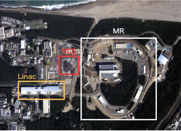
The Japan Proton Accelerator Research Complex (J-PARC) is located in Tokai Village, Ibaraki Prefecture, Japan [25]. J-PARC can provide the highest intensity proton beam in the world.

(26)

Linac

RCS

MR

Figure 2.2: Aerial photograph of J-PARC. The LINAC can accelerate protons up to 400 MeV, the RCS accelerates protons up to 3 GeV, and the MR can accelerate protons up to 50 GeV.

J-PARC consists of series of accelerators such as a LINAC that accelerates protons up to 400 MeV, a Rapid-Cycling Synchrotron (RCS) that accelerates protons up to 3 GeV, and a Main Ring (MR) that accelerates protons up to 50 GeV. The accelerated protons are used for multiple purposes, for instance in the materials and life science experiments such as non- destructive inspection using neutron diﬀraction, physics experiments using muons or neutrons, and so on. The MR protons are used for neutrino experiments or hadron experiments. The basic specifications of J-PARC are summarized in Table 2.1, and a schematic view of J-PARC is shown in Figure 2.2.

Accelerator LINAC RCS MR

Beam power 200 kW 1 MW 750 kW Beam repetition 25 Hz 25 Hz 0.3 Hz

Beam current 50 mA 333 µA 25µA Table 2.1: Basic specifications of J-PARC [25].

(27)

2.3.2 Materials and Life science experimental Facility

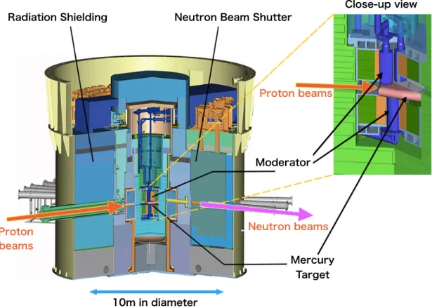
Materials and Life science experimental Facility (MLF) [26] is one of the multipurpose experimental facilities in J-PARC. In this facility, experiments on materials and life sciences, and fundamental physics using neutrons and muons are carried out. The MLF can provide the world’s highest-intensity pulsed neutron and muon beams for users. A schematic top-view of the MLF is shown in Figure 2.3. There are four muon beamlines and 23 neutron beamlines including those under construction. About 10% of the provided protons are used to generate muons, and the remaining protons are used to generate neutrons. A carbon target and mercury target are used for the muon and neutron sources, respectively. The neutron source is shown in Figure 2.4. This neutron source has three types of moderators: named coupled, decoupled, and poisoned, to provide neutron beams of various energies and intensities. The coupled and the decoupled moderators are classified according to whether they have a neutron absorber between moderator and reflector. The decoupled moderator has a neutron absorber, and it can provide a narrower width and less intense neutron pulse than that of a coupled moderator.

This moderator is suited for the analysis for material structures with a high resolution. On the other hand, the coupled moderator, which has a high intensity and wide pulse width, is suited for experiments that need high intensities. The poisoned moderator has an additional neutron absorber at a certain moderator depth. This moderator provides a neutron pulse that has a narrower width than that of the decoupled moderator provides. The mercury target is placed at the center of the neutron source, and it is surrounded by moderators. The mercury target and moderators are covered with a beryllium reflector, and they are placed within steel and concrete radiation shielding. Generated neutrons are sent into 23 beamlines, and are turned on or oﬀ by a shutter made of steel and polyethylene. Our experiment is being carried out at BL05, which uses a coupled moderator to obtain high-intensity neutrons.

(28)

Muon Line

Coupled De-coupled Poisoned Moderators :

Proton beams

Figure 2.3: Schematic top-view of the MLF. There are four muon beamlines and 23 neutron beamlines, including those under construction. Neutron beams are classified into three groups depending on the type of moderator.

(29)

Radiation Shielding Neutron Beam Shutter

Close-up view

Proton beams

Moderator

Neutron beams

Mercury  Target 10m in diameter

Proton   beams

Figure 2.4: Neutron source at the MLF. The mercury target is placed closest to the neutron source, and it is surrounded by three kinds of moderators. The mercury target and moderators are covered with a beryllium reflector, and they are placed within steel and concrete radiation shielding. The beam shutter is made of steel and polyethylene.

(30)

2.3.3 BL05 (NOP)

BL05 (NOP) is a beamline constructed for neutron optics and fundamental physics [27]. A schematic view of BL05 is shown in Figure 2.5. In BL05, in order to cope with the various experiments, cold neutrons provided from the neutron source of the MLF are divided into three beam branches. One of them is a low divergence beam branch, which is used for experiments requiring neutrons with a low divergence such as small-angle neutron scattering. Another beam branch is an unpolarized beam branch, which can provide the highest intensity neutron beam from BL05. This beam branch is used for UCN generation because it has advantages in terms of the statistics. The other one is a polarized neutron beam branch, which can provide highly polarized neutrons (>95% polarization) [28]. The specifications of each beam branch are summarized in Table 2.2. Our experiment uses the polarized neutron beam branch to reduce background events. The approach to background reduction will be discussed in the following section.

Low divergence Un-polarized Polarized

Beam size [mm²] 80×20 55×45 80×50

Beam divergence [µstr] 5.4×10⁻² 1.0×10² 1.9×10² Beam intensity [n/sec/cm²] 5.4×10⁴ 9.4×10⁷ 3.9×10⁷

Polarization – – >95%

Table 2.2: Specifications of each beam branch of BL05. The calculated values assume 1 MW operation of J-PARC, and 16 m from the moderator of the neutron source [25, 27, 28].

A

B C D BL06

BL04

Shielding

Figure 2.5: Schematic view of BL05. A : upstream beam bender, B : polarized beam branch, C : unpolarized beam branch, D : low divergence beam branch. The exit of each beam branch is located at 16 m from the moderator surface of the neutron source [27].

(31)

2.4 Experimental apparatus

In this section, our experimental apparatus will be explained. Our experiment has some unique features to obtain better statistics and less background events.

2.4.1 Setup

The setup for neutron lifetime measurement at J-PARC is shown in Figure 2.6. Neutron beams are formed as short bunches by using the Spin Flip Chopper (SFC). Then, these short bunches are transported into the TPC. The neutron flux is measured by the beam monitor, and neutron beam is turned on or oﬀ by the ⁶LiF shutter. The details of each device are described in the following sections.

Figure 2.6: Setup for neutron lifetime measurement at J-PARC. (A): shielding, (B): lead shields, (C): iron shields, (D): ⁶LiF beam collimators, (X): polarized neutron branch, (Y): un-polarized neutron branch, (Z): low divergence neutron branch, (a): wavelength filter, (b): guide coil, (c):

flipper coil, (d): magnetic super mirrors, (e): beam monitor, (1): Zr window, (2): ⁶LiF shutter, (3) veto counters, (4): lead shields, (5): vacuum chamber, (6): TPC, (7): ⁶LiF beam catcher, (8): turbo molecular pump.

(32)

2.4.2 Spin Flip Chopper

The SFC is the most unique device in our experiment [29]. This device can form the neutron pulse into short bunches by utilizing the neutron spin. A schematic top-view together with a photograph are shown in Figure 2.7. The SFC consists of two spin flipper coils, three magnetic super mirrors and a guide coil to hold the neutron polarization.

A B C D E

F G H

Figure 2.7: Schematic top-view (top) and the photograph (bottom) of the SFC. There are two spin flipper coils, three magnetic super mirrors, and a guide coil. A : first spin flipper coil, B : first and second magnetic super mirrors, C : ⁶LiF collimator, D : second spin flipper coil, E : third magnetic super mirror, F : guide coil, G : ¹⁰B absorber, H : lead shielding.

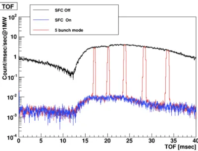
The spin flipper is a device for flipping the neutron spin using Larmor precession due to an oscillating magnetic field. The magnetic super mirror consists of thin alternating layers of ferromagnetic and non-magnetic materials, and it can reflect only neutrons that have the same spin direction as the direction of the magnetic field when placed in the magnetic field. The guide coil creates a static magnetic field in the SFC and prevents from depolarization of the neutron spin. By combining this equipment, the neutron pulse can be formed into neutron bunches. The time structure of the MLF beam and bunch structure of BL05 are shown in Figure 2.8. By using the SFC and the formed neutron bunches, it is possible to reduce the number of gamma ray background events caused by the neutrons while the neutron bunches pass through the detector.

(33)

Figure 2.8: Time structure of the MLF beam and bunch structure of BL05. The SFC forms the pulsed neutron beam into five bunches to minimize the number of background events caused by neutron hits on the TPC or other materials.

2.4.3 Beam monitor

A beam monitor is placed downstream of the SFC. In order to reduce the number of gamma ray background events, we use a ⁶LiF shutter, which will be described in the next section, to take data with and without neutrons introduced into the TPC. The beam monitor is used to normalize the neutron flux. We employ a detector manufactured by CANBERRA in which³He gas is filled. A picture of the beam monitor is shown in Figure 2.9.

2.4.4

⁶

LiF shutter

As mentioned in the previous subsection, by using the LiF shutter, it is possible to acquire both of data with neutrons and without neutrons. ⁶Li has a large neutron absorption cross section (940±4 barn [23]), and since the gamma ray emission probability due to neutron absorption is as small as 0.083%, neutrons can be dumped without increasing the number of gamma ray background events. We made a shutter using a 5 mm thick ⁶LiF plate (⁶Li is enriched up to 95% of the included Li), and about 99.98% of the neutrons can be dumped. The opening and closing of this shutter is remotely controlled using a stepping motor. Figure 2.10 shows a picture of the ⁶LiF shutter.

(34)

Figure 2.9: Picture of the beam monitor.

Figure 2.10: Picture of the ⁶LiF shutter. The white plate seen in the center of the photograph is a ⁶LiF plate.

(35)

2.4.5 Time Projection Chamber

The TPC is a type of gas detector and consists of a region that drifts electrons, which are ionized along with the passage of charged particles, by using an electric field and a Multi-Wire Proportional Chamber (MWPC) to detect the drifted electrons. The amplifiers to read out the electrical signal are mounted on the MWPC frame. A photograph of our TPC is shown in Figure 2.11. The size of our TPC is 960 mm in the beam axis direction, 300 mm in the vertical and the horizontal directions [30]. The TPC and MWPC frames are made of Poly-Ether-Ether- Ketone (PEEK) [31], which has low radioactive contamination. The wall surfaces of TPC are covered with tiles made of⁶LiF in order to reduce the number of gamma ray background events due to the neutron absorption reaction of the TPC wall as much as possible. These ⁶LiF tiles are also covered with Teflon to prevent alpha particle and tritium produced by the neutron absorption reaction of ⁶Li from entering the sensitive region of the TPC. There are two slits on one side for the calibration system. The slit positions are shown in Figure 2.12. The details of the calibration system will be described in the next section.

Figure 2.11: Photograph of the TPC. The frames of the TPC and MWPC are made of PEEK, which has low radioactive contamination. The amplifiers to read out the electrical signal are mounted on the MWPC frame. The wall surfaces of the TPC are covered with tiles made of

6LiF.

(36)

Figure 2.12: Inside photograph of the TPC. There are two slits on one side of the TPC for calibration.

We use⁴He as the working gas because it has small scattering and absorption cross sections, and we also use CO₂ as a quenching gas. The mixing ratio of these gasses is ⁴He:CO₂=85:15, and regular operations are carried out at the total pressure of 100 kPa. In the region shown in Figure 2.12, there is an electric field from the bottom to the top of the TPC for transporting ionized electrons. The MWPC has 24 channels of anode wire (applying 1720 V in 100 kPa operation) and 24 channels of field wire (applying 0 V) parallel to the beam axis, and 40 channels of cathode wire (applying 0 V) perpendicular to the beam axis. For the cathode wire, four or five wires merged into a channel. The alignment of each wire is shown in Figure 2.13.

The anode wires, field wires, and cathode wires are all sense wires. There are amplifiers on the top of the MWPC to read out the signal coming from drifted electrons and ions. The specifications of the TPC are summarized in Table 2.3.

Sensitive region 300 mm (horizontal)

×300 mm (vertical)

×960 mm (beam axis)

Anode wire ϕ 20µm Gold plated tungsten (AuW) Field wire ϕ 50µm Beryllium copper (BeCu) Cathode wire ϕ 50µm Beryllium copper (BeCu)

Anode channel 24 channels

Field channel 24 channels

Cathode channel 40 channels

Table 2.3: Specifications of the TPC

(37)

Figure 2.13: Alignment of each wire of the MWPC. Anode wires and field wires are aligned in parallel, and cathode wires are aligned perpendicular to the anode wires. Red lines are anode wires, blue lines are field wires and yellow lines represent cathode wires.

2.4.6 Calibration system

In our experiment, X-rays from ⁵⁵Fe are used as the calibration source of the TPC. This ⁵⁵Fe source is attached to the rotating stage, which is controlled by a stepping motor, and it is possible to irradiate X-rays into the TPC from slits opened at 75 mm and 225 mm from the bottom of the MWPC. The reason for using two slits is to evaluate the eﬀect of attenuation inside the TPC. During data acquisition, the calibration data at the near position (75 mm) and far position (225 mm) are collected once per hour.

2.4.7 Cosmic veto system

The cosmic veto system consists of several pairs of plastic scintillators, wave length sifters, and photomultiplier tubes. This system it the most eﬃcient at reducing the cosmic background.

This cosmic veto system covers the entire surface, except the bottom of the lead shielding of the vacuum chamber. The bottom surface of the vacuum chamber is supplemented by a plastic scintillator for the cosmic ray trigger, which is placed inside the lead shielding. According to the evaluation of the detection eﬃciency of this cosmic veto system, the detection eﬃciency for cosmic rays was more than 99%. The count rate of the cosmic background was reduced from 55 cps to 0.5 cps using this veto system. It is possible to acquire the cosmic events by reversing the veto condition, which is useful in calibrating the drift velocity of electrons in the TPC. At 100 kPa, it was typically 1.1 cm/µsec.

(38)

2.5 Data acquisition system

The data acquisition system of this experiment is shown in Figure 2.14. The signals on the wires of each event are recorded by a Flush Analog to Digital Converter (FADC) and Time to Digital Converter (TDC) [32] to obtain the waveform and time information, respectively. To reduce the number of background events from environmental gamma rays, the vacuum chamber that contains the TPC is covered with lead shields. Furthermore, in order reduce the number of background events due to cosmic rays, a cosmic veto system using plastic scintillators is placed around the lead shields. During data acquisition, a coincidence of hit on the anode wire and no hit on the cosmic veto system is used as the trigger.

Anode  or Field  or Cathode

Cosmic  Veto

Discri. 24ch OR Gate Gen. Gate Gen. Gate Gen.

Trigger

Waveform FADC

Self veto

Discri. 7ch OR Cosmic veto

Busy

TDC

Stop

Kicker  pulse

Start

Figure 2.14: Block diagram of the data acquisition system. The trigger signal is generated by a coincidence of hit on the anode wire and no hit on the cosmic veto system. The kicker pulse from J-PARC is used for the TDC start.

Since the FADC is working with 10 MHz sampling, the maximum time range of an event is 100 µsec, and when a cosmic ray event is observed by the cosmic veto, a dead time of 70 µsec is set. The time information of the kicker pulse corresponding to the timing of the proton colliding with the mercury target provided by J-PARC is used as the start signal of the TDC.

(39)

2.6 Simulation

The eﬃciencies for neutron β decay and neutron absorption by ³He, as well as the number of background events caused by scattered neutrons, are estimated using a Monte Carlo simulation.

The Monte Carlo simulation is carried out in two parts. The first part is a simulation of a particle interaction in the TPC by Geant4. In this part, various kinds of particle interactions are simulated, and their deposit energy, interaction point, and time are recorded. The second part simulates the response of the detector. The waveforms of all wires are simulated with information from Geant4. We take into account diﬀusion, recombination, and attenuation to convert the results of Geant4 to a waveform. This waveform has the same data format as that of the experimental data, therefore the same analysis code can be applied to the simulated data. A list of Monte Carlo samples is shown in Table 2.4.

Samples Types

Neutron β decay (on axis) Signal Neutron β decay (oﬀ axis) Background

3He(n, p)t reaction (on axis) Signal

3He(n, p)t reaction (oﬀ axis) Background

55Fe source (near) Calibration

55Fe source (far) Calibration

Cosmic ray Calibration

6LiF absorption Background CO₂ absorption Background Table 2.4: List of Monte Carlo samples.

2.6.1 Simulation of particle interaction

We simulated the entire experimental apparatus. Figure 2.15 shows a snapshot of the simulated apparatus. From the innermost part, the TPC, vacuum chamber, beam duct, lead shields, veto counter, and L-shaped iron shield are shown in Figure 2.15.

(40)

Figure 2.15: Snapshot of the simulated apparatus. From the innermost part, the TPC, vacuum chamber, beam duct, lead shields, veto counter and L-shaped iron shield are shown.

(41)

The parameters of particle simulation, such as the measured beam structure, pressure of the operating gas, temperature, and status of the⁶LiF shutter, are provided to the simulation.

This information is necessary to determine the probability of a particle interaction in the TPC.

Finally, we can obtain the deposit energy, interaction point, and time of each simulated event.

2.6.2 Simulation of the detector response

The detector response is calculated using the deposit energy, interaction point, and time simulated by Geant4. The drift process of an electron in the TPC, and its amplification process near the MWPC are simulated by taking into account diﬀusion, recombination, and attenuation in the operating gas. Finally, a waveform is generated for each wire with electrical noise and pedestal oﬀset. The gain of each wire and the drift velocity are adjusted to reproduce the experimental values using the calibration data.

2.7 Result of 100 kPa operations

We measured the neutron lifetime with 1% statistical uncertainty by the electron counting method during 100 kPa operations of the TPC by 2016. Although the details of the analysis flow will be described in a later chapter, we obtained the first result of τn = 896 ± 10(stat.) ⁺¹⁴₋₁₀(sys.) sec as a result of analyzing the data from 100 kPa operations. Figure 2.16 shows our result together with the plots in Figure 1.5. Through analyzing the data for 100 kPa,

1990 1995 2000 2005 2010 2015 Year 2020

Neutron Lifetime[sec]

870 875 880 885 890 895 900 905 910 915

0.6 sec

± UCN Storage : 879.6

2.0 sec

± Proton Counting : 888.0

Proton Counting method

UCN Storage method

Our result

Figure 2.16: Summary of neutron lifetimes for all three methods. The proton counting method is shown with squares and the UCN storage method is shown with circles. The statistical uncertainty of our result is around 1%, as shown in the figure with diamond.

(42)

we found that the largest uncertainty is due to the background events caused by neutrons scattered by the operating gasses. These background events are diﬃcult to distinguish from neutron β decay events, and the reason will be described in Section 3.1. The background events caused by scattered neutron are an important issue to be solved in order to improve our experimental accuracy.

(43)

(44)

Chapter 3 Studies for low gas pressure operation

In order to reduce the background events from scattered neutrons, we reduced the operating gas pressure of the TPC. In this chapter, we describe the results of the test operation of the TPC at low gas pressures and the development of a new amplifier.

3.1 Motivation for low pressure operation

Since various nuclides have scattering cross sections for neutrons, a certain number of neutrons are scattered by the operating gasses in the TPC. These scattered neutrons hit the wall of the TPC or the beam duct, and then gamma rays are generated by the (n, γ) reaction with a certain probability. If these gamma rays generate electron by Compton scattering, it can show up as a background event. An illustration of a background event caused by a scattered neutron is shown in Figure 3.1. Analyzing the data at 100 kPa, it was confirmed that the background events due to these scattered neutrons existed in about 5% of the β decay events. Thus, in order to realize the measurement with 0.1% accuracy, it is crucial to reduce the number of these background events. Since the operating gas has a certain neutron scattering cross section, it is possible to reduce the amount of scattered neutrons by reducing the absolute number of operating gas molecules. The scattering and absorption cross sections of He and CO₂ for neutrons are summarized in Table 3.1. The scattering cross section of CO₂ is approximately four times of that of ⁴He. These scattering cross sections are suﬃciently small compared to the other various nuclei; however, in order to achieve a measurement with 0.1% accuracy, it is necessary to remove the background caused by scattered neutrons.

Nuclei Scattering cross section [barn] Absorption cross section [barn]

3He 6 5333

4He 1.34 0

C 5.551 0.0035

O 4.232 0.00019

CO₂ 4.67 0.0013

Table 3.1: Scattering and absorption cross sections of various nuclei for 2200 m/s neutrons.

The values for C and O are calculated using the natural abundance of each nuclei, and the value for CO₂ is calculated using the molar ratio [23].

(45)

MWPC

TPC Drift direction

Beam  position

electron  from  beta decay

scattered  neutron

gamma ray

electron  from  gamma ray

Figure 3.1: Illustration of a background event caused by a scattered neutron. The scattered neutron hits the wall of the TPC and generates gamma rays with a certain probability. If these gamma rays generate electron by Compton scattering, it can show up as a background event.

The red dots at the MWPC represent anode wires, the green dots represent field wires, and the blue lines are cathode wires.

3.2 Test operation at J-PARC

In September 2016, we carried out a TPC operation test at low gas pressure at J-PARC. In this test, evaluation of the gain of the TPC by a ⁵⁵Fe source was performed. At this time, we did not use a neutron beam for the test.

3.2.1 Setup

In order to investigate the robustness of our TPC and optimize the data acquisition conditions at low gas pressures, the test was carried out under the conditions of 25 kPa of the mixture of

4He and CO2, and 15 kPa, 7.5 kPa, and 3.75 kPa of CO2 gas only. The data acquisition for only CO₂ gas is also for testing the feasibility of mono-gas mixture operation. To optimize the data acquisition, the high voltage applied to the anode wire was adjusted. This is because of Paschen’s law concerning spark discharge [33]. The Paschen’s law is represented using the gas pressure P and distance between electrodes d as

V = C₁P d

ln(C₂P d)−ln[ln(1 + _γ¹

se)] (3.1)

(46)

where V is the breakdown voltage, C₁ and C₂ are constants which are determined experimen- tally, and γ_se represents the secondary electron emission coeﬃcient. We reduced the voltage applied to the anode wire and adjusted it so that no discharge occurred for each gas pressure.

The voltage applied to the anode wire for each gas pressure is shown in the Table 3.2.

Gas pressure Voltage on anode wire [V]

4He + CO₂ 25 kPa 1180

CO₂ 15 kPa 1720

CO₂ 7.5 kPa 1400

CO₂ 3.75 kPa 1180

Table 3.2: Voltage applied to the anode wire for each gas pressure. The lower the gas pressure, the lower the voltage applied to the anode wire for the same gas mixture. The CO₂ 15 kPa corresponds to the amount of CO2 gas in 100 kPa of the mixture gas.

3.2.2 Gain evaluation

Using the configuration mentioned in the previous subsection, the evaluation of the gain of the TPC at low gas pressures was performed. A comparison of the gains at 100 kPa and 25 kPa is shown in Figures 3.2 and 3.3. The “near position” indicated in the figure means the data was taken with the slit that is the nearest to the MWPC, and “far position” means the data taken with the slit farthest from the MWPC. The transport eﬃciency represents the ratio of the gains of the near and far positions. It can be confirmed from Figures 3.2 and 3.3 that the gain of the TPC was 1/3 or less due to the decrease in the voltage applied to the anode wire to meet the decrease of the operating gas pressure.

(47)

ADC ch Deposit Energy with ⁵⁵Fe @ 100kPa

Far position Near position

Gain from Near Gain from Far

Figure 3.2: Gain at 100 kPa. The calibration source was ⁵⁵Fe and the voltage applied to the anode wire was 1720 V. The “near position” indicated in the figure means the data was taken with the slit nearest to the MWPC, and “far position” means the data was taken with the slit farthest from the MWPC. The transport eﬃciency represents the ratio of the gains of the near and far positions.

(48)

Deposit Energy with ⁵⁵Fe @ 25kPa

Far position Near position

Gain from Near Gain from Far

ADC ch

Figure 3.3: Gain at 25 kPa. The calibration source was ⁵⁵Fe and the voltage applied to the anode wire was 1180 V. The “near position” indicated in figure means the data was taken with the slit nearest to the MWPC, and “far position” means the data was taken with the slit farthest from the MWPC. The transport eﬃciency represents the ratio of the gains of near and far positions.

中性子寿命測定の高精度化に関する研究