Optimizing Chemical Plant Operation by Mixed Integer Programming

Society of Japan

Vol. 31, No. 1, March 1988

OPTIMIZING CHEMICAL PLANT OPERATION

BY MIXED INTEGER PROGRAMMING

Hiroshi Konno

Tokyo Institute of Technology

Hiroaki Sekino

Research Center, Mitsubishi Chemical Industries, Ltd.

(Received November 5, 1986; Revised March 25, 1987)

Abstract This paper addresses itself to the maximization of the yield of some chemical process subject to various operational as well as physical constraints. Some of the operational constraints on such factors as the level of flows and the number of flow change are discrete in nature and standard mathematical formulation leads to a medium scale mixed integer programming problem. A typical problem contains 150 integer variables in addition to 150 con· tinuous variables and 200 constraints. A problem of this size may not possibly be solved by the general purpose mixed integer programming code in accordance with our basic requirement, i.e., in less than one minute on 1 MIPS computer.

Thus we introduce a series of relaxation schemes by elaborating the special structure of the problem and reduce the original problem into a set of subproblems, all of which can be solved by standard methods.

We tested this algorithm on a number of real scale problems and always obtained almost optimal solution within 1 minute, whose discrepancy from the true optimum was less than 1 % relative to the value of the objective function.

1. Introduction

Let us consider an optimization problem associated with a chemical process depicted in Fig. 1, where some chemical by-product generated while processing main product in plant F is sent to plant A to recover its valuable ingredients. The capacity of plant A is relatively small compared to largely fluctuating input, so that it is temporarily stocked in the intermediate storage 5 before processed in plant A. The amount in excess of the capacity of the storage S will be burned in plant B.

We naturally want to maximize the amount of flow into plant A or equiva-lently minimize the amount to be sent to plant B. There are, however, several

45 constraints on the operation of each plant.

First of all, the level of flow into plant A can be adjusted only once a day.

Main product

bet) Intermediate yet)

by-product storage S Plant B

Plant F

!

x

Plan'

J

Fig. 1

The level of flow into plant B can be adjusted more frequently, typically as many as ten times every twenty-four hours, but it is preferred to have as few changes as possible primarily because too many changes will put excessive load on the operator. In addition, it must be integer multiple of some posi-tive constant. Also, lower and upper bound constraints are imposed on each variable.

The traditional operation of this system can be described as follows. We set the amount of flow into plant A at the level much lower than'the presumably best achievable value to avoid the fatal violation of lower bound constraint of the storage S. According to this scheme, we usually have to

(i) burn much more than necessary

(ii) change the level of flow into plant B intolerably ·often

which'motivated our present effort to optimize the operation using advanced mathematical programming technique.

We will formulate this problem as a mixed integer programming problem in Section 2. A typical discretization of the original continuous time problem leads to a mixed integer linear programming problem consisting of some 150 integer variables and 200 constraints. A problem of this size could not possibly be solved by a general purpose Dlixed integer programming code within one minute on 1 MIPS computer, which is the crucial requirement imposed on our solution strategy.

We therefore develop a special purpose algorithm in Section 3 where we incorporate a series of relaxations by exploiting the special structure of this problem. As shown in Section 4, our algorithm can generate an almost optimal solution for every input data we examined. It turned out that the difference of the value.of the objective function is always less than 1% from that of the true optimum. Also, we could significantly reduce the number of changes of flow into plant B.

There are only a few publications on the applications of mathematical programming techniques to the optimization of chemical process in our country, at least to our knowledge [2,3,5,7].

In particular, we could find almost no published reports on the applica-tions of mixed integer programming. We hope that this paper will call upon a new interest in the applications of mixed integer programming in this field.

2. The Model

Let bet) be an exogenous function representing the amount of flow into intermediate storage S at time t. Also, let

x

y (t)

z (t)

rate of flow into plant A

rate of flow into plant B at time t amount in storage S at time t

The following equation represents the flow balance at storage S d

dtz(t)

=

bet) - x - yet),

o ;;;

t ;;; T

z(O)

=

Zo

)

where T is the planning horizon, usually twenty-four hours. Lower and upper bound constraints are imposed on the variables:

0 ;;; x :;; x max (2) Ymin :;; y (t) ~~ Ymax ' 0 :;; t :;; T z min :;; z (t) ~; z max' 0 :;; t :;; T

1

Also, yet) should be an integer mUltiple of positive constant a, i.e.,. (3) yet)

=

w(t)·a ,

wet) LS a nonnegative integer for all t

}

Finally yet) should be a piecewise constant function with at most ten dis-continuous points. Our problem is to maximize the yield x subject to

constraints described above.

To solve this problem, we discretize time interval of 24 hours into L

minutes subintervals to obtain the following discretized version of equation (1)

(4) x + y. + a(z. - z. 1) = b.,

]

]

r

]

j=1 , •.• ,n

where n = 1440/L, a = I/L. Constraints on the number of discontinuities of

y(t) can be represented by introducing n zero - one variables as follows:

(5 ) Y_j - Y j-1 + mpj 6 0, -Y j + Yj-1 + mpj 6 0, n LP. ~ 10 j=1 ] P_j E {O,

n,

j=I, ••. ,n j=I, ..• ,n j=I, ••• ,n

where m is a large positive constant. It is easy to see that P

j Y_j

=

Y_j-₁ whereas P_j

=

1 implies

Y j - Y j-l ;;; -m

°

implies

which imposes no restriction on Y

j - Yj-1 when m is large enough, so that

constraints (5) judiciously represent our restriction on the number of dis-continuities.

(6)

Our problem can now be written as follows:

maximize x subject to x + y. + a(z. _. z. )

]

]

r

1

°

~ x ~ x _max Ymin ~ Yj ~ z min ~ z. ] ~ Yma.x ' zmax' w. ~ 0, integer, ] Y_{j -} Y_{j -1} + mp~i ;;; 0, -Y_j + Y_j-₁ + mp j ~ 0, n LP. ~ 10 j=1 ] P_j E {O, 1 }, j=I, ••• ,n j=I, ••• ,n j=I, ••• ,n j=I, •.• ,n j=I, ••• ,n j=I, ••• ,n j=I, ••• ,n j=I, ••• ,n

Typically when T=20(minutes! this problem contains about 150 integer variables in addition to 150 continuous variables. Also it has about 200 constraints other than lower and upper bound constraints on the variables. We are requested to supply an optimal yield x* and associated operation scheme within one minute after the input data b(t) is provided from the factory every morning.

3. Algorithmic Strategy

The problem formulated in Section 2 is a medium scale mixed integer programming problem which could not be solved in one minute on 1 MIPS computer by the state-of-the-art general mixed integer programming code. We are thus forced to devise an approximation of the model and a special purpose algorithm to solve a resulting approximate problem.

We will describe here a very successful relaxation strategy consisting of the following four steps.

[Step 1]

We will first relax the complicating constraints related to the number of discontinuities of Y .'s and solve the resulting linear programming problem:

] (7) Let ously x (8) maximize x subject to x + y. + a(z. - z. 1)

]

]

r

o ;;;

x ;;; x max Ymin ;;; Yj ;;; z min ;;; z. ] ;;; Ymax ' z max' b., ] x, Y j, Zj' j=l, •.• ,n be an optimal solution

gives an upper bound of the optimal solution x ;;:; x*

j=l, ••• ,n

j=l, ••. ,n

j=l, ••. ,n

of this problem.

Obvi-*

x of (6), i.e. ,

[Step 2]

We are slmost done if the number of discontinuities associated with

Y.'s

] are less than 10. It is, however, an exceptional case and we try to reduce the number of discontinuities by solving another subproblem:

n minimize

_{I 1}

Y ,

-

_{Y j-1}

1

j=1 J (9) subject to _{Y j} + a(zj

-

2 j_1 ) b, J

-

x, j=1, ••. ,n Ymin :;; Y j :;; Ymax ' j=1, ••• ,n 2 min :;; 2, J :;; 2 max, j=1, ••• ,n

It is straightforward to see that this problem has an optimal solution

Y

j, ~j' j=1, ••• ,n, which can be obtained by solving an equivalent linear

programming problem: n minimize

_I

(v ~ + v~) j=1 J J subject to _{Y j} + a(2 j

-

2, 1)

_r

(10) Ymin ~ _{Y j} ~ _Y max ' 2 :;; 2, :;; 2 max' m~n _J + - v, + v, J J v~;;;o,v,;;;o, J J [Step 3J b. - x, J 0, j=1, ••• ,n j=1, .•. ,n j=1, •.• ,n j=1, ••• ,n j=1, ••• ,n

Since we want to have as few discontinuities as possible, we will try to further reduce it. Let k be the number of discontinuous points associated with

Y

_j , j=1, .•• ,n and let j1' j2, . . . ,jk be the time at which the jump takes place. We will introduce k variables

n

1,

n

2, ...

,n

k, one for each interval on which Y ,'s are constant and rewrite the constraint of problem using these

J

k variables instead of y,'s. (See Fig. 2)

J

yet)

-i--

n₂

6---<0

~ n₄

?---9---<Q

.',. n ----'

ki

---<>

~---~---~'---~~---.I

Ir/---••

---4.~~.~

n Fig. 2

We thus solve a sequence of k linear programs LP(i) for i=l, •.• ,k:

minimize

subject to n; + a(z. - z. 1) = b. - x,

~

]

r

]

( 11) LP (i)

Ymin ~ n. ~ ~ Ymax ' i=l, ... ,k z ~ z j ~ z max' m~n j=l, .•. ,n ns

-

_ns-1 0, S E: J i where J

1=<P and Ji is recursively defined as follows:

if the optimal value of the objective function of LP(i) is zero

otherwise

If the resulting number of discontinuities is greater than 10, we have to gradually decrease the level of x from its best achievable value

x

and solve

(9) again until this requirement is satisfied (Fortunately, this routine was not activated for all test problems.)

Let j1' j2,···,jp be points of discontinuities of Yj'S, where p ~ 10. [Step 4]

Solve the following mixed integer program generated from (6) by fixing p

time points jl, ..• ,jp at which jump of Y_j is possible.

maximize x subject to x + _Ys + a(z.

-

z. 1) b. ]

r

] js + 1 ~ j ~ js+l ' s=l, ... ,p (12) 0 ~ x ~ x max Ymin ~ Ys ~ Ymax ' s=l, ... ,p z min ~ z. ] ~ z max' j=l, ... ,n Ys = integer multiple of a, s=l, ... ,p This problem contains less than ten integer variables Y

s' s=l, •.. ,p so that it can be solved by standard branch and bound technique. We will employ the optimal solution (x, Yl""'Yp' ~l""';n) of (12) as our approximate optimal

Plant Operation

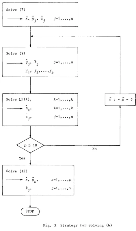
Fig. 3 shows the flow chart of our solution strategy. Note that each subproblem (7), (9) and (12) are significantly easier than (6).

Solve (7)

-

-

-•

x, Yj' z. j=l, .•• ,n ] Solve (9) ~ ~

•

Yj' z . _] j=l, ••• ,n j l' j2' .. • ,jk LP(£),

I

-

-

oj

Solve £=1, .•• ,k x :

₌

x

-~ • n£, £=1, ••• ,k

-Zj' j=l, ••• ,n No Yes Solve (12)

-•

x, Ys ' s=l, .. • ,p

-Zj' j=l, ..• ,n

(

STOP

4. Computational Results

We first compared our solution strategy with the traditional method which

~s based upon the experience and intuition of the operator ~n charge of this system. Table 1 summarizes the result where T=60(minutes) in all four cases.

Table 1

Attained yield x (9, /hr) Number of jumps of Y j

,

s Traditional

New method Traditional New method

method method

Case A 154.0 170.8 5 2

Case B 152.0 164.4 7 2

Case C 162.8 171.6 6 2

Case D 164.8 181.7 9 2

This table shows that our method always generates a solution whose yield

~s about 10% better than the traditional method. Also the number of jumps is remarkably less.

We next applied our method to the typical input data depicted in Fig. 4.1 where T=20(minutes). Fig. 4.1 shows the optimal solution of (7) and Fig. 4.2 shows the optimal solution of (9). Note that the number of discontinuities of

y(t) dropped from 12 in Fig. 4.1 to 3 in Fig. 4.2. Fig. 4.3 shows the solu-tion after solving k linear programs LP(9,), 9,=1, ••• ,k where the number of discontinuities decreased even further. Fig. 4.4 shows the optimal solution of (12) where ~ is greater than 0.99~. We thus obtained a feasible solution of (6) in which; satisfies

x*

f;

x

~ 0.99x* by noting (8).

Optimizing Chemical Plant Operation 53 ~ 0 0

,.,

0

"'

N b(t) 0 -:; 0 N <:'. ~ ~ ~ S;

'"

0 ~ y(t) 0

"'

0 0 4 12 16 20 24 TIME (hr) Fig. 4.1 Ca) 0

"'

,.,

0 0 '" 0

"'

N 0 z(t) 0 N ~ .... 0 :> 0 ~ 0 ~ 0

"'

0 0 8 12 16 20 24 TIME (hr) Fig. 4.1 Cb)

0

"'

M 0 g 0 ~ 0 -;:; 0 N

e

:'j

]

0

'"

~ 0

::

0

"'

0 0 0

"'

M 0 0 M 0

"'

N 0 0 N

3

c; :> 0 ~ 0 ~ 0

"'

o 8 8 12 TIME (hr) Fig. 4.2 12 TIME (hr) 16 Ca) 16 Fig. 4.2 Cb) b(t) y(t) 20 24 Z(t) 20 24

55 0

"'

..,

0 0

..,

0 "' N b(t) 0 ';:; 0 N .:::.

.::

) ~ 0 .... ~ 0 S 0

"'

_y(t) 0 0 8 12 16 20 24 TIME (hr) Fig. 4.3 Ca) 0 :q 0 0

..,

0

"'

N 0 z (t) i'l :; ~ 0 > 0

"'

0 S 0

"'

0 0 12 16 20 24 TIME (hr) Fig. 4.3 Cb)

0

"'

"'

0 g 0 ~ b(t) 0 0:- i'l ~ ~ !> ~ _~

..

0 ~ 0

"'

y(t) 0 0 B 12 16 20 24 TIME (hr) Fig. 4.4 Ca) 0 :q 0 0 "' 0

"'

N 0 z (t) 0 ~ N .-< 0 0-0 ~ 0 0 ~ 0 0 12 16 20 24 TIME (hr) Fig. 4.4 Cb)

57

Table 2 shows some of the more important constants used Ln our

computa--

-tion. Table 3 shows the value of x and x for four different input data. We observe from this that the difference fron x* are less than 1%. Also, we observe from Table 4 that the number of discontinuities is less than 3 Ln each case. (See in particular a remarkable success in Case 4.)

Every result shows the validity of our solution strategy. It should be emphasized that these remarkable success 'Nas not expected at all before we started this study since T=20(minutes) problem has been too complicated to obtain a reasonably good operation scheme by traditional approach based on experience and intuition.

Table 2. Physical Constants

x _Ymin Y_max a z . Z T

max mLn max

200 40 100 5 140 260 20

(£/hr) (£/hr) (£/hr) (£/hrj (£)

(n

(min)

Table 3. Attained Yields Table 4. Number of Flow Change

~(£/hr) ;U/hr) x/x

-

-

Step 1 Step 2 Step 3

Case 1 187.4 186.8 0.997 Case 1 8 3 3

,

Case 2 172.0 171. 7 0.998 Case 2 5 4 2

Case 3 162.8 161.5 0.993 Case 3 12 4 3

Case 4 155.9 154.7 0.992 Case 4 14 3 3

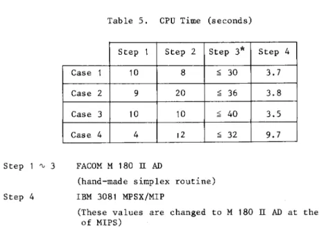
Finally, Table 5 shows the amount of time required to obtain this solu-tion, which successfully meets the computational requirements.

We expect from these results that this method can solve an even larger problem with smaller T (say 5 minutes) or l.onger planning horizon (say 1 week) by

(i) using more elaborate implementation technique instead of the rudimentary upper bounded simplex method currently in use eii) skipping the most time consuming St.ep 3 and instead using the

best least square approximation procedure [6] of a piecewise constant function by another piece.rise constant function with a fixed number of jumps.

Step 1 'V 3

Step 4

Table 5. CPU Time (seconds)

Step 1 Step 2 Step 3*

Case 1 10 8

Case 2 9 20

Case 3 10 10

Case 4 4 12

FACOM M 180 IT AD

(hand-made simplex routine) IBM 3081 MPSX/MIP ;£ 30 ;£ 36 ;£ 40 ;£ 32 Step 4 3.7 3.8 3.5 9.7

(These values are changed to M 180 IT AD at the rate of MIPS)

* Include overhead jobs. Real execution time is considerably less.

Acknowledgement

Part of the research of the first author was supported by Grant-in-Aids for Scientific Research of the Ministry of Education (A) 5900004.

References

[1] Chvatal, V.: Linear Programming, Freeman and Co., 1983.

[2] Hikosaka, T.: A New Advanced Energy Center Computer System ~n Steel Works. (in Japanese), Iron and Steel, Vol.64, No.13 (1978), 82-91.

[3] Kashiwagi, M.: Energy Management System of a Chemical Plant. (in Japanese), Sho-Energy, Vol.34, No.l0 (1982), 25-31.

[4] Konno, H. and H. Suzuki (eds.): Integer Programming and Combinatorial

Optimization. (in Japanese), Nikka Giren Publishing Co., 1982.

[5] Hatsunaga, K.: Optimal Allocation of Energy in an Iron Mill. (in

Japanese), Heat Management and Industrial Pollution, Vol.28, No.l (1976), 29-34.

[6] Konno, H. and T. Kuno: Best Piecewise Constant Approximation of a Func-tion of Single Variable. Abstracts of the Spring Meeting of the Opera-tions Research Society of Japan, 1987.

[7] Nishio, M., K. Shiroko and T. Umeda: Optimization of Fuel Supply in a Chemical Plant. (in Japanese), Comm. of the Operations Research Society

59

of Japan, 27, 344-350 (1982).

Hiroaki SEKINO: Mathematical System Laboratory, Research Center,

Mitsubishi Chemical Industries, Ltd. '1000, Kamoshida, Midori-ku, Yokohama, Japan.