パノラマ距離画像からの路上駐車車両の検出
8
0
0
全文
(2) I. INTRODUCTION In crowded urban areas, street-parking vehicles occupy a certain area of the streets at any time and cause traffic problems, such as impediment to the traffic flow and blind spots. In Japan, 1,800,000 parking tickets are issued annually. Among them, 480,000 parking tickets are issued in Tokyo alone. Illegal parking is a common problem in metropolises as indicated by the number of tickets issued annually, e.g., 10,000,000 in New York, 4,000,000 in London, and 2,800,000 in Seoul [1]. In the United States and Europe, both police and local governments clamp down on illegal parking. In case of the local government, the criminal status of illegal parking is reduced or removed. In Japan as well as England, there is a plan to entrust the control of illegal parking to the private sector before long [2]. Nevertheless, illegal parking is not decriminalized. Information about street-parking vehicles is useful for re-planning roads and traffic system. In Japan, street-parking vehicles have to be manually counted by investigators in measuring vehicles during traffic-condition survey. Manual counting faces problems, such as human error and high cost. Feasible street-parking-vehicle counting system in term of accuracy and cost is desired for privatization and effective traffic census. We previously proposed the detection method by a scanning laser-range finder (LRF) [3]. However, occlusion such as from a vehicle going past the measurement vehicle leads to incorrect detection. The detection method is available only off-line and needs large data storage. We proposed also an alternative detection method [4], based on an epipolar-plane image (EPI) analysis, which are easily obtained by a line-scan camera. EPI analysis, firstly developed by Bolles [6], is a technique for building a 3-D description of a static scene from a dense sequence of images. EPI analysis is used to calculate the features depth from the slope of feature paths in EPIs. However, the method is applicable during daytime and it needs much processing time. Sakuma et al. [5] proposed the counting method by detecting wheels. The method creates panoramic images and extracts vehicles’ wheels by morphological processing to those panoramic images. It is applicable only during daytime. Its cost is high because it generates a panoramic image from multiple 2-D frames. A long belt of scene along streets is profiled continuously, from which street-parking vehicles are extracted. Zheng [16] provided ‘digital route panoramas’, which is a new image medium for digitally archiving scenes along a route. However, object detection is out of his league.. Zhao et al. [14], [15] proposed a vehicle-borne system of measuring 3-D urban data. The system uses single-row laser range scanners, line cameras and a vehicle positioning system. The laser range scanners construct vertical range profiles for measuring object geometry and horizontal range profiles for tracing vehicle location and orientation [15]. The line cameras measure the texture of the urban features [14]. The detection method proposed in this paper is based on cluster analysis, from panoramic street range-images obtained by a scanning LRF [7]. A processing at each scan is repeated, and can detect vehicle clusters. The proposed system is economical, robust to occlusion and applicable all day long. The detection method is simple. First, panoramic street-image will be addressed. Second, the detection method will be presented with experimental results. Conclusion and future works will be described.. II. SPATIO-TEMPORAL VOLUME In this section, panoramic street images will be introduced from spatio-temporal volume images. Panoramic street images are the combination of 2-D panoramic-view images and 3-D panoramic-range images. Panoramic street images are used for detecting objects as well as vehicles parked on streets. A. Spatio-Temporal Volume Two important cases in object detection are the detection of moving objects from a stationary camera and vice versa. In the first case, image subtraction and background subtraction are often used. In the latter case, motion stereo is often used for extracting 3-D information from 2-D images of stationary objects. This paper focuses on detection of stationary objects by a sensor with lateral motion. Lateral motion is illustrated in Fig. 1. While the sensor (for example, a camera) moves laterally, a target P is projected to points P1 , P2 and P3 on the camera’s image plane at time T1 , T2 and T3 , respectively. The plane on which there are the target P and arbitrary two camera optical centers, is called an epipolar plane. The epipolar plane intersects two corresponding image planes along an epipolar line. Epipolar lines on the image plane for a lateral motion are collinear and parallel to the camera optical center’s trajectory.. -2−42−.
(3) P Feature Point PVI. Epipolar Line P3. EPI Vertical Pixel [pixel] (spatial domain). P2 P1. Image Plane. C3 t3. C2 C1 Trajectory of Camera Optical Center. feature point P is projected to points P1 , P2 and P3 in the image plane, at time, T1 , T2 and T3 , respectively. Our algorithm considers a 3-D spatio-temporal volume, which is a multiframe array generated by concatenating multiple image frames along the time domain. The multiframe array is a 3-D volume in a spatio-temporal domain [8], [9]. The camera moves laterally, the background also sweeps across multiple image frames. In this case, two important 2-D images can be generated from a 3-D spatio-temporal volume. The two images are derived by slicing a 3-D spatio-temporal volume: (1) an epipolar-plane image (EPI) from horizontal slicing [10], and (2) a panoramic-view image (PVI) from vertical slicing. The result of the slicing process is shown in Fig. 2. The front plane of the 3-D spatio-temporal volume is the first frame. Its side plane is a panoramic-view image. Its top plane is an epipolar-plane image. A panoramic-view image and an epipolar-plane image are created by slicing the spatio-temporal volume, vertically and horizontally, respectively.. Vertical Pixel [pixel] (spatial domain). side top 66. 10310 10260. front 10210 294. 10160 10110 10060. Horizontal Pixel [pixel] (spatial domain). 700. 10010. (a). 10160 10110. Horizontal Pixel [pixel] (spatial domain). Fig. 1 Lateral motion of camera. A camera optical center is located at points C1 , C2 and C3 , and a. 360. 10210 294. 10060. 360. Time. 486 20. 10310 10260. First Frame. 486 20. t2 t1. PVI. EPI. 66. Frame Number (time domain). 700. Frame Number (time domain). 10010. (b) Fig. 2 Spatio-temporal volume representation: (a) Spatio-temporal volume generated by concatenating multiple images along the time domain. The first frame is the front plane. Panoramic-view image is the side plane. Epipolar-plane image is the top plane. (b) Panoramic-view image and epipolar-plane image are created by slicing the spatio-temporal volume, vertically and horizontally, respectively.. B. Line-Scan Imaging PVIs and EPIs are generated by concatenating specific line-images in each image frame; PVIs from specific vertical line-images and EPIs from specific horizontal line-images. A line-scan camera with lateral motion is enough to create PVIs or EPIs. Line-scan cameras are based on line-scan imaging technology and provide other benefit than area-scan cameras (frame cameras). Perhaps the most common example of line-scan imaging is the fax machine. Line-scan imaging uses a single line of sensor pixels (effectively one-dimensional) to build up a two-dimensional image. The second dimension results from the motion of the object being imaged. Two-dimensional images are acquired line by line by successive single-line scans while the object moves perpendicularly past the line of pixels in the image sensor. Line-scan imaging has some benefits, including (1) dynamic range that can be higher than conventional cameras, (2) smear-free images of fast moving objects, and (3) processing efficiency: line scanning eliminates the frame overlaps required to build a seamless image, particularly in high-speed, high-resolution applications. C. Panoramic Street Image A laser range finder (LRF), used in line-scan imaging, realizes one more dimension. The third dimension results from the measurement of the distance up to objects. Three-dimensional images are also acquired line by line while the object moves. -3−43−.
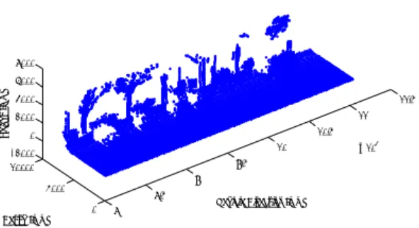
(4) perpendicularly past the scanning line. When the line-scan sensor moves, instead of objects, perpendicularly to the scanning line, line-scan imaging is also realized and the same benefits can be received. Line-scan imaging system mounted on a measurement vehicle exploits its abilities, when it runs at a high speed in the outdoor environments. By using a line-scan camera, two-dimensional and seamless images are easily acquired, and on the other hand, a LRF generates three-dimensional and seamless images, as shown in Fig. 3. Panoramic street-image has 3-D information by two methods: one method is the extraction of depth information from EPI, and the other is .the restoration of 3-D information using LRFs. Both methods use line-scan imaging technology effectively.. 3D Distortion of Laser Range Data. 8000 Height [mm]. 6000 4000. 11.5 11. 2000 10.5. 0 10. -2000. 4. x 10. 9.5. 10000 9. 5000. 8.5 0. Depth [mm]. 8. Vehicle Direction [mm]. Fig. 3 Panoramic street range image using a laser range sensor when it scans vertically. A. Three Dimensional Restoration The data of panoramic street range-images are originally obtained in the 2-D polar-coordinate system, with its origin at the sensor. It is more desirable to store them in the 3-D coordinate, which is easy-to-understand format. Fig. 3 shows one such 3-D restoration of range data. The laser beam cannot travel through objects, except the transparent/semi-transparent. Objects located nearer the laser sensor occlude objects further away. Higher emplacement of a LRF can be positioned to tilt downward towards street-parking vehicles, and prevent occlusion of the street-parking vehicles. B. Compensation of LRF’s Tilt Each vertical-scan of a LRF provides a sectional plane of panoramic street range-images, perpendicular to the street, as shown in Fig. 4. The LRF should be mounted carefully, but in practice, it cannot be free from tilting. Such tilt is responsible for inclining a road surface in the 3-D range-images. In order to realize a road surface as the horizontal plane, this tilt of the LRF needs to be compensated. A laser beam from the LRF fans out from bottom to top, and a few first laser beams are likely to hit on a road surface. The tilt angle of the LRF can be calculated from range-points hitting on the road surface. After the compensation of the tilt angle at each scan, a road surface can be reconstructed as a reference horizontal plane with the level 0. It is easy to understand a 3-D scene by visualizing range-points data, as shown in Fig. 4, and to simplify a further process, an analysis and an implementation.. Those images include much and useful information for our everyday life, such as: 1) Barrier-free facilities, such as steps between sidewalks and streets, that must be monitored on the way to an aging society, 2) Road-use real situation, like street-parking vehicles and derelict bulky garbage, 3) Road-traffic facilities, installed in the road traffic environments and public spaces, including traffic signs and road-side trees.. scanNo.288. 9000. 8000. 7000. Infinity. Higher Region. Height [mm]. 6000. 5000. 4000. 3000. Bush (cluster 2). Height 2000mm. 2000. Sidebody (cluster 1) 1000. Road Surface 0. This paper is focused on the detection of street-parking vehicles, using Cluster analysis.. III. DETECTION USING CLUSTER ANALYSIS Panoramic street range-images can be acquired by a vertical-scanning LRF mounted on the measurement vehicle moving in a lateral motion. The detection method from these range-images is described in this section.. -1000 9000. 8000. 7000. 6000. 5000. 4000. 3000. 2000. 1000. 0. Depth [mm]. Fig. 4 Range points plotted on the depth-height graph at no.288 scan.. C. Selection of Region of Interest To detect street-parking vehicles, it is sufficient to. -4−44−.
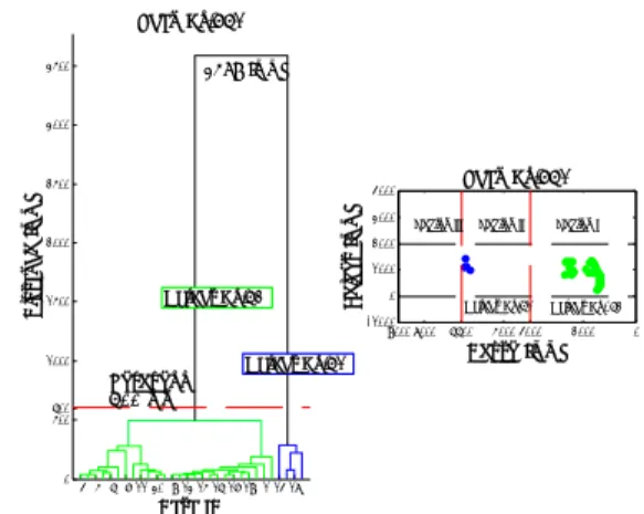
(5) D. Intra-Scan Clustering Range points in the ROI are desired to construct clusters for every object, at each scan. Firstly, for measuring the similarity between every pair of range points, the Euclidean distance dij between every pair are computed. When pairs of range points are in close proximity, they are grouped together into binary clusters. The newly formed clusters are grouped into larger clusters until a hierarchical tree is formed. A hierarchical, binary cluster tree is created by using the nearest-neighbor-algorithm, which uses the smallest distance between objects in the two groups, R and S , d ( R, S ) = min {dij } . i∈R , j∈S. The hierarchical, binary cluster tree is plotted as a dendrogram graph, as shown in Fig. 5. In the dendrogram graph, the height of the linkage line indicates the distance between objects. Range points in the hierarchical tree are divided into clusters by cutting off the tree at a threshold distance. The threshold for cutting the dendrogram graph is 600 mm, indicated by a red line in Fig. 5. Two clusters were created; a green one indicated a vehicle’s moving past the measurement vehicle, and a blue one indicated a street-parking vehicle stopping at the side of a road.. E. Inter-Scan Clustering Inter-scan clustering groups the result of the intra-scan clustering (intra-clusters) with the intra-clusters of the previous scan and forms the inter-cluster. In inter-scan clustering process, the average depth of every intra-cluster is calculated. If intra-clusters from the consecutive scans have the average depth difference less than 500 mm, they are grouped into the larger inter-cluster. When the subsequent scan has no cluster to be merged into the intra-cluster, the inter-cluster stops growing, and is called the object-cluster. Scan No.761 3500. 3589 [mm]. 3000. 2500. 2000. 1500. Scan No.761. 4000. Object No.62. Height [mm]. Distance [mm]. limit the analysis to a specific region, called region-of-interest (ROI). ROI is a region with its height less than 2000 mm, and is neither a road surface nor a region beyond measurement range. Vehicles run on the ground, don’t take off, and can be safely assumed to have the height of less than 2000 mm. Range points more than 2000 mm, red dots in Fig. 4, can then be ignored. After compensation of the LRF’s tilt, a road surface can be regarded as a horizontal plane, with its level at 0 mm. When measurement error is taken into account, it is reasonable to assume that a road surface has an absolute value of its height less than 100 mm high. Range points at the height of less than 100 mm (black dots in Fig. 4) are not considered. In our experiments, the LRF can measure objects up to 8000 mm away, and returns a range value of 8191 mm for the object beyond. These limits draw the arc with radius 8191 mm at the center of the LRF, blue dots in Fig. 4. Only the ROI which is determined as mentioned above, is considered. Street-parking vehicles will be detected in the ROI.. 3000. Region III. 600 500. 0. Object No.61. Region I. 1000 0 -1000 9000 8000. 1000. Region II. 2000. Object No.61 6600. Object No. 62. 5000 4000. 2000. 0. Depth [mm]. Threshold 600 mm. 4 5 6 7 11 30 9 13 15 16 17 19 1 14 18. Data ID. Fig. 5 Dendrogram graph and range-point clusters at no.761 scan. Three Regions After creating the object-clusters based on the intraand inter-clustering, one vehicle may be divided into two object-clusters. To prevent the construction of too small object-clusters, ROI is divided into three regions, and the smaller object-cluster is merged into the larger object-cluster, if the smaller object-cluster is always in the same region as the larger one. Three regions are determined based on the experiment and the width of the lanes. In our experiments, the measurement vehicle traveled on the rightmost lane in the three-lane street. Three regions are determined as follows; Region I with depth from the LRF less than 4000 mm, Region II with depth from 4000 mm to 6600 mm, and Region III with depth over 6600 mm, as shown in Fig. 5.. -5−45−.
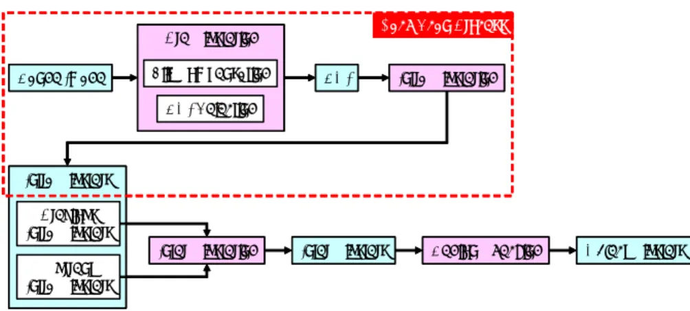
(6) Each Scan Process. Pre-Clustering Range Image. Tilt-Compensating. ROI. Intra-Clustering. ROI-Selecting. Intra-Clusters Previous Intra-Clusters Inter-Clustering. Inter-Clusters. Region Checking. Object-Clusters. Current Intra-Clusters. Fig. 6 Detection diagram of object-clusters indicating street-parking vehicles. F. Detection of Street-Parking Vehicles Intra-clustering, inter-clustering and region-checking can group range points into the real objects. The whole process is summarized in Fig. 6. In these experiments, objects in Region III are regarded as a bush or something at the edge of roads. Objects in Region I are regarded as street-parking vehicles, and objects in Region II are regarded as vehicles moving between the measurement vehicle and the street-parking vehicle. G. Experiments The LRF was mounted on the measurement vehicle as shown in Fig. 7. The measurement vehicle traveled at the speed about 40 km/h. From Region I, 5 vehicles were detected among 5 vehicles going past. From Region II, 36 vehicles from 40 street-parking vehicles were detected correctly. There was a case that two street-parking vehicles were merged incorrectly into one vehicle, and this case occurred twice. These 4 vehicles were regarded as non-detected vehicles. On the other hand, all of 5 street-parking vehicles which were partially occluded by vehicles going past the measurement vehicle, were correctly detected. The detection results are summarized as a confusion matrix in TABLE 1.. TABLE 1 Confusion matrix of detection results predicted actual negative positive. negative. positive. N/A 4. 0 36. Fig. 8 illustrates the experimental results of vehicle extraction from panoramic street-images obtained by the line-scan camera.. (a). (b) Fig. 7 The line scan camera and the laser range sensors mounted on our measurement vehicle. (a) the whole of the vehicle and (b) the line-scan camera and the scanning laser range finders.. IV. CONCLUSIONS. The accuracy of this system/method is 36 per 40, 90%. Precision is 36 per 36, 100%. True positive rate, that is, recall rate is 36 per 40, 90%. The detection rate is calculated as ‘accuracy’ in this paper, and, thus, 90%.. We introduced the spatio-temporal volume and its two slice surfaces, PVI and EPI. Furthermore, we derived the two-type panoramic street images: one image uses intensity data from a camera, and the other uses range data from a LRF. The panoramic street images were obtained by vertically scanning line-scan. -6−46−.
(7) camera and laser range sensor. They include much and useful information for our daily life. We proposed the method for detecting street-parking vehicles: the method is based on cluster analysis. In the detection method based on cluster analysis, its detection rate achieved higher 90 %. In addition, this method indicated its robustness to partial occlusion. Future Work A laser sensor can measure the distance directly and robustly in the outdoor environment. However, an image sensor like a camera has much more information from data. Thus, we will fuse an image sensor and a laser sensor, and improve the whole system. After extracting vehicles images from the panoramic street image, vehicle classification will be the next task.. ACKNOWLEDGMENT This work was partially supported by ITS division, the Research Center for Advanced Information Technology, the National Institute for Land and Infrastructure Management (NILIM), the Ministry of Land, Infrastructure and Transport (MLIT), Japan. The authors thank Dr. S. Auethavekiat in the University of Tokyo.. 2D Spatio-Temporal Image Transformation Technique”, Proc. Int’l. Conf. Intelligent Transportation Systems, pp.634-638, 1999. [9] P. Wang, K. Ikeuchi and M. Sakauchi, “3D Line’s Extraction from 2D Spatio-Temporal Image Created by Spline Slit”, Proc. Asian Conf. Computer Vision, vol.II, pp.408-415, 1998. [10] Z. Zhu, G. Xu and X. Lin, “Panoramic EPI Generation and Analysis of Video from a Moving Platform with Vibration”, Proc. Conf. Computer Vision and Pattern Recognition, pp.531-537, 1999. [11] H. Zhao and R. Shibasaki, “A Vehicle-Borne Urban 3-D Acquisition System Using Single-Row Laser Range Scanners”, IEEE Trans. Systems, Man, and Cybernetics Part B: Cybernetics, vol. 33, no. 4, pp.658-666, 2003. [12] H. Zhao and R. Shibasaki, “Reconstructing a Textured CAD Model of an Urban Environment Using Vehicle-Borne Laser Range Scanners and Line Cameras”, Int’l. J. Machine Vision and Applications, vol. 14, no. 1, pp.35-41, 2003. [13] J. Y. Zheng, “Digital Route Panoramas”, IEEE Multimedia, vol. 10, no. 3, pp.57-67, 2003.. REFERENCES [1] The Asahi Shinbun, “Clampdown on Illegal Parking Is Privatized”, Column ‘Keizai-Kishou-Dai’, June 10, 2003 (in Japanese). [2] “Fixed-Point Observation”, Car and Drivers, vol.26, no.10, Diamond Publisher, 2003 (in Japanese). [3] S. Ono, M. Kagesawa and K. Ikeuchi, “Parking-Vehicle Detection System By Using Laser Range Sensor Mounted on a Probe Car”, Proc. Intelligent Vehicle Symposium, 2002. [4] C. Zhu, K. Hirahara and K. Ikeuchi, “Street-Parking Vehicle Detection Using Line Scan Camera”, Proc. Intelligent Vehicle Symposium, pp.575-580, 2003. [5] S. Sakuma, Y. Takahashi, A. Shio and S. Ohtsuka, “Vehicle Counter System Using Panoramic Images”, IEICE Trans. Information and System, vol. J85-D-II, no. 8, pp.1361-1364, 2002 (in Japanese). [6] R. C. Bolles, H. H. Baker and D. H. Marimont, “Epipolar-Plane Image Analysis: An Approach to Determining Structure from Motion”, Int’l J. Compute Vision, vol.1, pp.7-55, 1987. [7] K. Hirahara and K. Ikeuchi, “Detection of Street-Parking Vehicles Using Line Scan Camera and Scanning Laser Range Sensor”, Proc. Intelligent Vehicle Symposium, pp.656-661, 2003 [8] C. Li, K. Ikeuchi and M. Sakauchi, “Acquisition of Traffic Information Using a Video Camera with. -7−47−.
(8) 9000. 0. 500. 1000. 1500. 2000. 2500. 3000. 7000. 6000. 5000. 4000. 3000. 2000. 1000. 0. 8.3. 8.4. 8.5. 8.6. 8.7. Depth [mm]. 7000. 6000. 4000. 3000. (h). Depth [mm]. 5000. 2000. 1000. 0. 2.25. 2.26. x 10. 5. Distance [mm]. 2.27. Distance [mm]. x 10. 4. (d). 9000. 0. 500. 1000. 1500. 2000. 2500. 3000. 8000. 8000 7000. 6000 5000. Depth [mm]. 7000. 4000 3000. 1000. (i). 2000. 0 2.57. 2.58. 2.6. 6000 5000 4000. x 10. 2.61. 5. 3000 2000. (e). Depth [mm]. Distance [mm]. 2.59. ObjectNo.76 (From scanNo.870-880, 706points, avgDepth=4896.18). 9000. 9000. 8000. 0. 500. 1000. 1500. 2000. 2500. 3000. 0. 500. 1000. 1500. 2000. ObjectNo.61 (From scanNo.761-764, 30points, avgDepth=6286.47). 8000. (c). Height [mm]. 2500. 1000. 9000. 0. 500. 1000. 1500. 2000. 2500. 3000. 0. 9. Distance [mm]. 9.1 x 10. 9.2. 4. 7000 6000. 4000 3000. Depth [mm]. 5000. 2000. (j). 1000 0. 2.61. 2.62. ObjectNo.77 (From scanNo.881-887, 272points, avgDepth=6324.7). 8000. 8.8. 8.9. ObjectNo.3 (From scanNo.300-306, 220points, avgDepth=5352.22). 2.63. x 10. 5. (f). 0 9000. 500. 1000. 1500. 2000. 2500. 3000. 7000 6000 5000. 9000. 0. 500. 1000. 1500. 2000. 2500. 3000. 8000. 4000. 7000. 3000 1000 0. 2.21. 2.22. 2.23. Distance [mm]. 2.24. 2.26. 2.27 5. 5000 4000. Depth [mm]. 6000. 3000 2000 1000 0. 3.02. (k). 3.03. 3.04. 3.06. Distance [mm]. 3.05. 3.07. (g). 2.29. x 10. 2.28. ObjectNo.90 (From scanNo.1020-1039, 944points, avgDepth=5942.42). 2000. 2.25. ObjectNo.59 (From scanNo.748-771, 2616points, avgDepth=1474.77). Depth [mm]. 8000. Distance along the ro. g. 5. 3.08. x 10. -8-. Fig. 8 Panoramic street images and range-point clusters of each vehicle. (a) and (b) Panoramic street images acquired by serial scans. (c) Range-point cluster of the first street-parking vehicle in (a). (d) Street-parking vehicle image cut off from (a) using the detection result (c). (e) Range-point cluster of the second street-parking vehicles in (a). (f) Street-parking vehicle image cut off from (a) using the detection result (e). (g) Range-point cluster of the vehicle going past our measurement vehicle. (h) Range-point cluster of the street-parking vehicle occluded by the vehicle (g). (i) Range-point cluster of the vehicle coming in from the road shoulder. (j) Range-point cluster of the vehicle occluded by the vehicle (i). (k) Range-point cluster of two street-parking vehicles.. Height [mm]. (b). Height [mm]. 3000. Height [mm]. (a). Height [mm]. ObjectNo.2 (From scanNo.283-293, 224points, avgDepth=4859.39). Height [mm]. −48−.
(9)
図

関連したドキュメント
調査の対象とした小学校は,金沢市の中心部 の1校と,金沢市から車で約60分の距離にある
13 proposed a hybrid multiobjective evolutionary algorithm HMOEA that incorporates various heuristics for local exploitation in the evolutionary search and the concept of
水平方向設計震度 機器重量 重力加速度 据付面から重心までの距離 転倒支点から機器重心までの距離 (X軸側)
駐車場 平日 昼間 少ない 平日の昼間、車輌の入れ替わりは少ないが、常に車輌が駐車している
• Mirrors, window lift, doors switches, door lock, HVAC motors, control panel, engine sensors, engine cooling fan, seat positioning motors, seat switches, wiper control,
11 特定路外駐車場 駐車場法第 2 条第 2 号に規定する路外駐車場(道路法第 2 条第 2 項第 6 号に規 定する自動車駐車場、都市公園法(昭和 31 年法律第 79 号)第
鉄道駅の適切な場所において、列車に設けられる車いすスペース(車いす使用者の
敷地からの距離 約48km 火山の形式・タイプ 成層火山..
