北九州市立大学 学術リポジトリ(ルクソール)

A Fully Synthesizable, Low Voltage and

Low Power Stochastic Flash A/D Converter

with Wide Input Range

September 2020

Department of Information Engineering The University of Kitakyushu

Author: Zou Xuncheng (Advisor: Shigetoshi Nakatake)

CONTENTS

CONTENTS...I

1. Introduction... 1

1.1 Background and motivation... 1

1.2 Thesis content and structure...10

2. Analog-to-Digital Converter... 12

2.1 Working Processes...12

2.1.1 Sample and Hold...13

2.1.2 Quantification... 14

2.2 Main Specifications of ADC...15

2.2.1 Basic Specifications...15

2.2.2 Static Specifications...17

2.2.3 Dynamic Specifications...20

3. Stochastic Flash ADC (SFADC)... 24

3.1 Principle...24

3.2 Number of Comparators Required...27

3.2.1 Theoretical derivation...27

3.2.2 Solution with uniformly distributed comparator offset... 32

3.2.3 Numerical Monte Carlo simulation... 35

4. Fully Synthesizable Rail-to-rail Dynamic Comparator... 40

4.1 Review and Proposed Rail-to-rail Dynamic Comparator...41

4.1.1 Review... 41

4.1.2 Proposed Rail-to-rail Dynamic Comparator...43

4.2 Simulation...47

4.3 Chapter Summary... 55

5. Linearity Enhancement Technique (LET)... 56

5.1 Prior Works...56

5.2 Our proposed Linearity Enhancement Technique (LET)... 60

5.2.1 Description of LET...62

5.2.2 The reduction in the number of comparator groups... 66

5.2.3 The determination of the number of comparators... 67

5.3 Effect of the proposed linearity enhancement technique...67

6. Implementation and Simulation... 74

7. Conclusion...78

CHAPTER 1

Introduction

1.1 Background and motivation

Recent advances in technologies of sensors, wireless communication and embedded processors have enabled the design of small-size low-power and low cost devices that can be networked or connected to the Internet [1]. These are the key components of the emerging paradigm of Internet-of-things (IoT) [2,3]. A few examples of such applications are wireless sensor networks, biomedical and implantable devices/networks, ambient intelligence, wearable computing, smart grids, pollution monitoring, plant monitoring, smart warehouses [4-6]. The applications explicitly rely on the availability of sensor nodes that are energy autonomous and extremely small sized [7]. It can be said that the booming development of the Internet of Things is inseparable from the low-power and miniaturization of electronic devices.

Low-power has emerged as a principal theme in today’s electronics industry. The need for low power has caused a major paradigm shift where power dissipation has become as important a consideration as performance and area [8].

v(t) i(t)

P(t)  _{(Eq. 1.1)}

where i(t) is the instantaneous current provided by the power supply, and v(t) is the instantaneous supply voltage [9]. When we discuss the battery life or the energy dissipation of the system, we are more concerned about the average power consumption over a period of time. At this time, assuming that the voltage is constant, reducing the average current can reduce the average power consumption of the electronic device. In addition, intuitively, lowing the supply voltage can also reduce the power consumption of a circuit.

Specifically for CMOS circuits, power dissipation is caused by three sources: 1) the leakage current which is primarily determined by the fabrication technology, consists of reverse bias current in the parasitic diodes formed between source and drain diffusions and the bulk region in a MOS transistor as well as the subthreshold current that exists at the gate voltages below the threshold voltage, 2) the short-circuit current (crowbar current) which is due to the DC path between the supply rails during output transitions and 3) the charging and discharging of capacitive loads during logic changes[8].

The power consumption induced by the leakage current is also called static power consumption; The total power consumption caused by the short-circuit current and the charging and discharging of capacitive load is called dynamic power consumption.

Static power consumption is the product of the device leakage

current and the supply voltage. Total static power consumption, PS,

can be obtained as shown in (Eq. 1.2).

voltage) (supply

current) (leakage

Ps 



The short-circuit power consumption component is less intuitive to be modeled because it depends on both the technology and the design parameters. It depends on the threshold and supply voltages, the drive strength of the gate, the frequency of operation, the input slope, and the output load connected to the gate [10]. A closed form for a symmetric inverter with the assumption of zero load capacitance at the output was derived was proposed as (Eq. 1.3) in [11] : clk T dd sc β (V V ) τ f P   ₂ 3  12 (Eq. 1.3)

where PSC represents the short-circuit power dissipation, β represents

the strength of the transistors, VT and Vdd are the threshold and

supply voltages, respectively, τ is the input slope, and fclk is the

frequency of operation. It has also a strong dependency on the ratio between the supply and threshold voltages.

The short-circuit and leakage currents in CMOS circuits can be made small with proper circuit and device design techniques [8]. The dominant source of power dissipation is thus the charging and

discharging of the node capacitances (also referred as the switching power dissipation) and is given by:

clk dd

sw / C V E(sw) f

P _{1 2}  2   _{(Eq. 1.4)}

Where C is the physical capacitance of the circuit, Vdd is the supply

voltage, E(sw) (referred as the switching activity) is the average

number of transitions in the circuit per 1/fclk time, and fclk is the clock

frequency.

In summary, supply voltage scaling seems to be a good approach for power optimization, since the power normally yields

considerable savings thanks to the strong dependence of power on

supply voltage Vdd. However, the lower supply voltage means the

lower circuit speed. Designers will have to make a trade-off between power consumption and circuit speed.

As the process continues to become more advanced, this contradiction has been alleviated. According to Moore's law [12], the number of transistors in an integrated circuit (IC) doubles about every two years, revealed in Fig. 1.1 [13]. The improvement of the process makes the feature size smaller. Also, the gate oxide of the MOSFET becomes thinner. The breakdown voltage of the device decreases, so the power supply voltage also decreases. The historic trend [14] in supply voltage is shown in Fig. 1.2.

Fig. 1.1: A semi-log plot of transistor counts for microprocessors against dates of introduction, nearly doubling every two years [13].

For digital circuits, the impact of low supply voltage on speed is offset by decreased gate capacitance. Therefore, process advance is conducive to power optimization for digital circuits. However, for analog circuits, the issue caused by low supply voltage can be big.

First of all, the primary index of the analog circuit is the signal-to-noise ratio. Lowering the supply voltage means that the signal swing is reduced, but the noise does not decrease in synchronization with the supply voltage. Therefore, low supply voltage has an adverse effect on the signal-to-noise ratio. Secondly, the threshold voltage of the device will not decrease synchronously with the supply voltage due to leakage, which makes the traditional circuit structure (such as cascode) no longer be adaptive at low supply voltage. Finally, since the threshold voltage does not decrease synchronously with the supply voltage, the operating region of the device is closer to the sub-threshold under low supply voltage, which is adverse to the linearity of the analog circuit.

In addition to the issues caused by the low supply voltage, the price of unit area in the advanced semiconductor manufacturing process is very high, but the overall size of analog circuits does not shrink proportionally with the reduction of feature size (especially passive devices, such as inductors, whose size has nothing to do with the feature size). Hence, the cost of analog circuits actually rises under the advanced semiconductor manufacturing process.

Consequently, digital circuits are more beneficial in scaling down than analog circuits. The use of digital circuits to replace analog circuits as much as possible can enjoy the benefits of process advances. Many related researches have been done, such as all-digital PLL, all-digital LDO, all-digital OPAMP, synthesizable RF transmitter [15-18].

Analog-to-digital converter (ADC) is an indispensable component in SOC. It almost represents the highest level in integrated circuit design, and has always been the focus and hot topic in IC field. Analog signals in the real world, such as temperature, pressure, sound and image, need to be converted to a digital form, which contributes to storing, processing or transmitting generally. ADC plays a role of a bridge between analog world and digital world. An analog signal comes into ADC, and a digital result would be generated.

ADC converts an analog value to a digital code according to specified rule. According to the difference in working mechanisms, it evolves into various of structures, including flash ADC, pipelined ADC, SAR ADC, ΣΔ ADC. Each has its own merits in speed, power, resolution, input bandwidth or other performance. Fig. 1.3 shows the comparison of several kinds of ADCs in regard to resolution and sampling rate. Compared to the other ADC, flash ADC is known for its high speed. Its resolution is usually between 4 to 9 bits, and the

operating frequency ranges from 10KHz to 10GHz. It is widely used in modulator, radio receiver, flash memory and so on.

Fig 1.3: Comparison of ADCs in regard to Resolution & Speed

However, it is difficult for conventional flash ADC to achieve higher resolution. The reason is that every time the resolution of one bit is increased, the number of comparators will double. Moreover, accomplishing the transformation from analog to digital needs comparator, which plays an important role in ADC. However, the device mismatch induced by process variation results in comparator offset, which affects the linearity of transfer function of ADC. As the process becomes finer, the feature size is increasingly reduced, making the offset voltage of the comparator more and more difficult

to overcome, thus the comparator offset is becoming one of critical factors for designer to design a good ADC.

To deal with issues of the comparator offset, some of researches had been done to reduce or cancel the comparator offset using special techniques [19-21]. There are two kinds of methods in general. One is adopting large size device, which exchanges chip area for small offset. The other is utilizing calibration. However, both of them cost a large design overhead inevitably. Therefore, a stochastic ADC [22] comes into being, which aggressively makes use of the comparator offset variability rather than leaving nothing to do.

Targeting a flash architecture based on the idea of the stochastic ADC, the prior work in [23] has analyzed a cumulative distribution function (CDF) of offsets among a lot of comparators induced by the process variation, and presents a stochastic flash ADC (SFADC), proposing a conversion mechanism to employ an approximately linear section of the cumulative distribution function as the transfer function.

However, there are two main problems we have to deal with in the SFADC. First issue is power. In order to express the probability through the number of comparators whose output is logic one, the SFADC needs a mass of comparators (far more than a conventional flash ADC) to meet the statistic requirements. Hence, if single comparator is not power-effective, the overall power will be very

high. The second problem is input range. In the configuration of [23], input-output transfer function is approximately linear only within the input range from -1σ to +1σ of comparator offset standard deviation. The input range of the SFADC is limited due to the bad linearity. In order to improve the signal-to-noise ratio of the ADC, it is necessary to broaden the linear range as much as possible.

Therefore, this work focuses on SFADC, and revolves around how to solve these two problems. And it is committed to propose a low supply voltage, low power consumption SFADC with a wide input range.

1.2 Thesis content and structure

In view of the superiority of SFADC under the deep sub-micron process size, we present a fully synthesizable SFADC, which can operate at the supply voltage of 0.6V with power consumption as low as 1.5mW at the clock frequency of 250MHz. By employing the all-digital comparator, the SFADC can be described with Verilog language and synthesized according to a standard digital design flow. Cross-coupled dynamic comparator structure saves the overall power due to remarkable control of dynamic power consumption. In addition, the rail-to-rail characteristic of comparator and the proposed linearity enhancement technique based on SFADC, allow us to design a wide-range SFADC.

The rest of the thesis is organized as follows. Chapter 2 introduces ADC’s theoretical overview and some of significant specifications. Chapter 3 mainly introduces the fundamental and properties of SFADC, and discusses the relationship between the number of comparators and signal-to-noise-and-distortion ratio. Chapter 4 is devoted into describing the fully synthesizable rail-to-rail dynamic comparator in our work. Chapter 5 elaborates the proposed linearity enhancement technique (LET). Chapter 6 illustrates the structure of the proposed SFADC and shows the advantage on power consumption, supply voltage and input-range based on simulation results. Chapter 7 concludes this work.

CHAPTER 2

Analog-to-Digital Converter

2.1 Working Processes

From an analog value which is continuous in time and amplitude, to a digital value which is discrete in time and amplitude, signal usually needs to go through four processes -- pre-filtering, sampling, quantization, and encoding, as shown in Fig. 2.1. Pre-filter filters the parts of signal outside the Nyquist frequency, to avoid aliasing caused by high frequency signal in the baseband of AD converter. Hence the pre-filter also can be called ‘anti-aliasing filter’. A S&H (Sample and Hold) circuit is connected to the anti-aliasing filter. A sampling circuit produces a sequence of δ functions of which amplitudes are equal to the ones of signal at the sampling times. Next, the holding circuit maintains the sampling signal, and makes it remain unchanged during the transformation. Then quantizer divides

reference voltage into 2N_{-1 sub-domains (N is the number of digital}

output bits). After finding out which sub-domain the sampling signal corresponds to, digital encoder begins to encode and outputs a digital result. In a transformation period, a sampling of the analog input signal is converted to an equivalent digital output code.

Fig. 2.1: A basic working process of ADC

2.1.1 Sample and Hold

Sampling is an operation of converting continuous time signal to discrete time signal. Ideally, sampling operation generates a pulse sequence whose amplitudes are equal to signal’s amplitudes at sampling points. Then holding operation maintains the sampling signal, and makes it remain unchanged during the transformation,

generating an analog signal xs(n*Ts) whose time is discrete and

amplitude is continuous, as shown in Fig. 2.2. Ts is the sampling

cycle and n*Ts (n = 0, 1, 2, ...) is called sampling moment.

Assume that fm represents highest frequency of input signal, and

1/(2*fm) is called Nyquist interval. Only if the sampling interval Ts is

less than the Nyquist interval 1/(2*fm), the sampling signal xs(n*Ts)

can be restored to the original analog input signal x(t), which is called Nyquist–Shannon sampling theorem.

2.1.2 Quantification

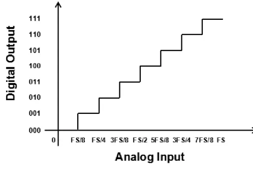
Quantification is an operation of converting continuous amplitude signal to discrete amplitude signal. Taking an ideal 3-bit ADC as an example, its transfer function is shown in Fig. 2.3.

Fig. 2.3: Transfer function of a 3-bit ADC in quantification

Input signal is an analog value from 0 to the FS (Full Scale), and

is divided into 2N_{subintervals. The width of subinterval is defined as}

the least significant bit (LSB), namely 1LSB = FS/ 2N_{. The trip}

points of transfer function are at x = k * LSB (k = 1, 2, ...). Similarly, digital to analog conversion also can be easily implemented. Each

digital bit (bx) has a weight of 2x-1, and a digital value can be restored

into an analog value as (Eq. 2.1).

2 2 2 2 2 0 1 1 2 2 1 1 _{b * ... b* b* ) LSB/} * LSB*(b V N N N N analog    _      (Eq. 2.1)

2.2 Main Specifications of ADC

2.2.1 Basic Specifications (1) Sampling Frequency

Sampling frequency is the reciprocal of the sampling time, and represents the times of conversion from continuous analog signal to discrete digital signal per second in the AD converter. The unit is Hz.

(2) Resolution

Resolution is the number of digital bits to represent an analog input. The resolution, together with reference voltage determines the minimum detectable voltage.

(3) Nyquist Frequency

Nyquist frequency, decided by Nyquist–Shannon sampling theorem, is the maximum bandwidth of input signal, which is equal to half the sampling frequency. If the maximum frequency of input signal is beyond the Nyquist Frequency, energy information of signal at different frequency can’t be restored with digital output signal.

(4) Input Signal Range

Input signal range is the quantitative range of ADC, generally determined by reference voltage. If the input signal is beyond the range of input, the AD converter will cause distortion.

(5) Power Consumption

Power consumption is energy consumed by AD converter per unit time when ADC works. Now low power consumption has become an important index in the ADC designing.

(6) Area

is the area of ADC on chip, often expressed in mm2_{, which}

2.2.2 Static Specifications (1) Offset

The offset describes an output shift for zero input, also expressed as shift error. It is the skewing of transfer function of ADC, expressed in mV or percentage of full scale. As shown in Fig.2.4, all of quantization levels shift an offset error.

Fig. 2.4: Offset error

(2) Gain Error

Gain error is the difference between the ideal analog input signal and the actual analog input signal when input causes a transition to full scale, expressed in the mV or the percentage of full scale, as

shown in Fig. 2.5. Another measure of gain error is the error on slope of transfer characteristic curve relatively to the ideal characteristic curve around the origin of coordinates. Unlike DNL and INL, both of gain error and offset error are linear error.

Fig. 2.5 Gain error

(3) Quantization Error

Quantization error is defined as the difference between ideal N-bit ADC output and infinite resolution converter’s output, also known as the least effective bit error. The analysis of quantization noise seems difficult since the quantization noise is a function of the input signal. Fortunately, under some specific conditions, quantization error can be approximate to white noise irrelevant to the input signal.

correspondence. When the input changes, the output may not change. Quantization error is innate in the AD converter, and is the lower limit of ADC error. Usually the only way to reduce the quantization error is improving resolution.

(4) Common Mode Error

is applied to differential inputs ADC, which represents the changes on output code when common mode input changes by a given value. It is usually measured by measuring the changes on equal common mode inputs when output code changes by 1 LSB, expressed in LSB generally.

(5) Differential Non-linearity Error (DNL)

is the step difference between actual transfer function and ideal one, expressed usually in LSB. Often the maximum DNL is simply referred as DNL. Differential non-linearity error can be expressed by (Eq. 2.2). LSB LSB LSB,x x _V V V DNL   _{(Eq. 2.2)}

where VLSB,x is the actual LSB

(6) Integral Non-linearity Error (INL)

Integral non-linearity error (INL) is the deviation of actual transfer function from endpoint fit line, usually expressed in LSB. Often the maximum INL is simply referred as INL. Integral non-linearity error can be expressed by (Eq. 2.3).



is the impedance between ADC inputs. The input impedance performs as resistance at low frequency. Ideally, input impedance of ADC is infinite when inputting voltage, and zero when inputting current. At high frequency the input impedance is usually determined by capacitive devices. As the switched capacitors are usually used in the ADC sampling, input impedance of ADC should match to input terminals at high frequency.

(2) Signal-to-noise Ratio (SNR)

Under the specific input and sampling frequency, ratio between the ADC output signal power and noise power is defined as signal-to-noise ratio. It is the ratio of ADC output signal and signal-to-noise without consideration of the distortion. For an ideal ADC, the SNR can be expressed as (Eq. 2.4). )(db) Noise Signal ( SNR 10log _{(Eq. 2.4)}

The input signals are generally sine waves when measuring. When only the quantization noise is considered, the signal-to-noise ratio of an ideal N-bit ADC can be calculated as (Eq.2.5).

(db) . N . SNR602 176 _{(Eq. 2.5)} (3) Signal-to-noise-and-distortion Ratio (SNDR)

Signal-to-noise-and-distortion ratio is referred to the ratio between the AD converter output signal power and the sum of all noise and harmonic power, generally expressed in dB. The calculation formula is revealed as (Eq. 2.6). )(db) Harmonics Noise Signal ( SNDR  10log _{(Eq. 2.6)}

(4) Total Harmonic Distortion (THD)

Total harmonic distortion is the ratio between total harmonic power and fundamental wave power within a specific frequency range, defined as (Eq. 2.7).

(db) ) Signal Distortion Harmonic Total ( THD  10 log (Eq. 2.7) (5) Effective Number of Bits (ENOB)

ENOB of AD converter is a dynamic value changing with signal frequency, and it reflects the effective conversion bits at different signal frequency in dynamic working.

With the increasing of input frequency, the overall noise (also distortion) will increases, thus reducing the ENOB and SNDR. So ENOB is often defined by SNDR as (Eq. 2.8).

6.02 SNDR-1.76

ENOB  _{(Eq. 2.8)}

and SNDR is expressed in dB. (6) Dynamic Range

is the value of input signal when SNR (or SNDR) becomes zero, usually expressed in dBFS (Full Scale).

(7) Spurious Free Dynamic Range (SFDR)

SFDR is defined as the ratio between RMS (root mean square) of input signal amplitude and RMS of the largest distortion component in first Nyquist domain. It is the difference value between component of fundamental wave (expressed in dB) and the highest noise component (expressed in dB) in the output spectrum. SFDR depends on the amplitude of input signal. For large input, the highest distortion is usually a harmonic component, but when the signal amplitude gets smaller, the distortion caused by the signal can be ignored. At this time, the distortion is often determined by other source rather than input signal. It is expressed as (Eq. 2.9).

(db) ) Harmonic or Spurious Largest Signal ( SFDR 10log _{(Eq. 2.9)}

For any good INL AD converter, SFDR is greater than SNR. Noise and harmonic are main factors limiting dynamic range of AD converter, thus SFDR is a very important specification for AD converter.

(8) Effective Resolution Bandwidth (ERBW)

Effective resolution bandwidth is referred to the frequency of input signal when SNDR of ADC decreases by 3 dB relatively to low frequency.

(9) Figure of Merit

Above specifications of ADC affect each other, so it is difficult to use a particular specification to measure the overall performance of the ADC. Now a common practice is taking the main performance parameters of ADC as a comprehensive index, and it is called FoM (Figure of Merit). The smaller FoM value is, the better the performance is. It can be calculated as (Eq. 2.10).

s ENOB_*f Power FoM 2  _(Eq.2.10)

Power is the total Power consumption of ADC; fs is the sampling

CHAPTER 3

Stochastic Flash ADC (SFADC)

3.1 Principle

In a conventional flash ADC, input signal is connected to input ports of a group of comparators. The reference voltage of each comparator is set precisely by reference ladder, so that all comparator thresholds are equally spaced by 1 LSB.

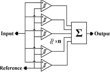
However, different from conventional one, as shown in Fig. 3.1, in the SFADC, an input signal line and a common reference voltage are connected to the inputs of comparators. Plus, following on the heels of a group of comparators, a Wallace Tree adder [24] is used to sum up the number of logic ‘1’ from all comparator outputs.

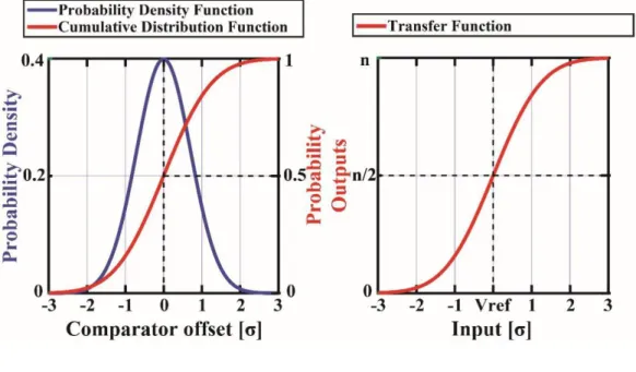
In a SFADC, the occurrence of comparator offset is not a drawback any longer, but rather something available. Due to device mismatch or processing variation, comparator offset appears to be random. The variation of comparator offset can be assumed to be a

Gaussian distribution with a mean (μ) of zero and variance (σ2₎

which is inversely proportional to the comparator area [25], as shown in Fig. 3.2(a). When a reference voltage is applied to the comparator, the comparator offset’s probability density function (PDF) becomes the PDF of Gaussian distribution with a mean of reference voltage, expressed by (Eq. 3.1).

 





The Wallace Tree adder counts for the number of high level voltage (i.e. logic ‘1’) in the outputs of comparators. As a result, when a ramp signal is given to a SFADC, the output of Wallace Tree adder is the cumulative distribution of a Gaussian distribution with a mean of reference voltage, as shown in Fig.3.2(b). In other words, the transfer function of a SFADC is regarded to be the cumulative distribution function (CDF) of the random comparator offsets, expressed as (Eq. 3.2).





 

_

_

_e

_dt

π

x

2

erf

If the amount of comparators is large enough, the PDF of comparators offset can be approximated to a Gaussian distribution function, as well as the conversion function is the CDF of Gaussian distribution. The mid-point of the conversion function is precisely corresponding to the reference voltage. In general, a conventional

N-bit flash ADC needs 2N_{-1 comparators, however, far more}

comparators must be incorporated into a SFADC to get closer to CDF of Gaussian distribution. SFADC’s transfer function has a good linearity between -1σ to +1σ (σ is the standard deviation of comparator offset). Thus the SFADC without calibration generally works in this input range.

(a) (b)

3.2 Number of Comparators Required

3.2.1 Theoretical derivation

Assuming that for any comparator i, the comparator offset’s

probability density function is Poffset,i. When an input voltage of v is

given to it, the output Di follows the Bernoulli distribution, whose

probability mass function Pv(Di) is expressed as (Eq. 3.3).

i i D i D i i v

(D

)

F

(v)

[

F

(v)]

P

_

_

₁

_





(v)

P

(V

)dV

F

If a SFADC contains N comparators in total, since the offsets of each comparator are independent of each other, the sum of the N comparator outputs (that is, the total output code D) represents the sum of N independent Bernoulli trials. D is given by (Eq. 3.4),





D

D

which follows a Poisson binomial distribution.

The exact PDF of the total output code D can be calculated by convolving the output codes of all the comparators, which is a huge

computation of the order O(2N_{) [26]. Even so, we can still use the}

first 2 moments to approximate the PDF of D to a curve in the Pearson family of distributions [27]–[28]. The first and second moment about 0 of D is given as (Eq. 3.5) and (Eq. 3.6), respectively.











where M1 also represents the mean μD of output code D at the input

voltage of v.

Only when all the comparators have the same Poffset, the

distribution of the total output code D will become a binomial distribution. At this time, the output code D has a probability mass function of (Eq. 3.7). D N D v

_D

F(v)

[

F(v)]

N

(D)

P

_















1



Then the first and second moment about zero of D is simplified to (Eq. 3.8) and (Eq. 3.9), respectively.

F(v)

N

μ

]

F(v)

)

[(N

F(v)

N

M









1





1

where μD is the average output code, which is a function of the

input v. In fact, it represents the average transfer function of SFADC. It should be emphasized that (Eq. 3.5) and (Eq. 3.6) are the general case of (Eq. 3.8) and (Eq. 3.9), regardless of whether the PDF of the comparator offset is same.

For an SFADC without calibration, only the relatively linear region in the transfer function can be used for ADC conversion. Let L(v) be the ideal linear portion in μD, that is, the expected output.

Next we define the quantization error qe as the difference between

the expected output L(v) and the actual output D, namely

D

v

L

q



(

)



Therefore, the variance of the quantization error qe can be derived

as follows. 2 1 2 0 2 0 0 2 2 2 0 2 0 2 2 2 2 M M L(v) L(v) (D) P D (D) P D L(v) (D) P L(v) ) D L(v) D (L(v) (D) P D) (L(v) (D) P ] E[q N D v N D v N D v N D v N D v e                      











(1) When all comparators have the same PDF of F(v), (Eq. 3.11) can be reduce to (Eq. 3.12) combining (Eq. 3.8) and (Eq. 3.9).

2 2

2

2_{] (N N) F(v) [2 N L(v) N] F(v) L(v)}

E[qe          (Eq. 3.12)

(2) When only the linear portion about v is contained in μD, in

other words, when L(v) is equal to μD, (Eq. 3.11) can be simplified to

(Eq. 3.13) combining (Eq. 3.5) and (Eq. 3.6).









]

F

(v)

[

F

(v)]

E[q

₁

(3) When the conditions of (1) and (2) are met at the same time, (Eq. 3.11) can be further reduced to (Eq. 3.14).

F(v)]

[

F(v)

N

]

E[q







1



The quantization noise energy Q is expressed as the integral of E(qe2) over the entire input range R, namely





]dv

E[q

Q

A ramp signal can be described as a random variable with a uniform PDF [29]. The variance of a random variable is equivalent to its mean-square power, and since the variance of a uniform PDF is found to be

12

2

Δ )

where Δ is the range of the PDF.

The signal energy S in the output is uniformly distributed between L(a) and L(b), where a and b are the start and end points of the linear input range R respectively. The signal energy S in the output is equal to the integral of the mean-square power over the entire input range of [a, b]. a) (b L(a)] [L(b) S     12 2 (Eq. 3.17)

Finally we can calculate the SNDR as (Eq. 3.18) combining (Eq.3.15) and (Eq. 3.17).



Although (Eq. 3.18) is still very complicated, we can draw some

useful conclusions. Firstly, for both L(v) and E[qe2], according to the

definition of L(v) and (Eq. 3.11), it is not difficult to find that they

are all related to μD, which is uniquely determined by the number of

comparators N and the offset’s distributions Poffset,i. Secondly, both

numerator and denominator of (Eq. 3.18) are related to the input range [a, b]. Therefore, SNDR is decided by the input signal range, the distribution of comparator offset, and the number of comparators. In addition, since SFADC usually works in a linear input range, for a given linear input range [a, b], L(v) can be replaced by

approximately μD. Thus the numerator S is proportional to N2. In the

same way, E[qe2] can be calculated by (Eq. 3.13), so the

denominator Q is proportional to N. As a result, the ratio of S and Q, SNDR is proportional to the number of comparators N. It indicates that every time the number of comparators is increased to 4 times of the original number, SNDR is also increased to 4 times. When

converted into dB, SNDRdB will increase by 6dB. According to

(Eq.2.8), the ENOB is increased by one bit.

3.2.2 Solution with uniformly distributed comparator offset

The general solution from (Eq. 3.18) is applied to two special cases in which comparator offset is uniformly distributed.

(1) Assume that comparator offset is randomly and uniformly distributed along full-scale from 0 to 1, namely

1

1 



/Δ

(v)

P

v

F(v) 

Then according to (Eq. 3.7), the probability mass function of the output code is

  



When a random uniformly distributed input is applied to this SFADC, according to (Eq. 3.8), the mean of the output code is N*v,

that is, the average transfer function is μD=N*v. It can be seen that

the average transfer function does not have a non-linear portion about v, so the expected output code is also L(v)=N*v.

The variance E[qe2] of the quantization error qe is found in

(Eq.3.14), that is, N*v*(1-v). According to (Eq. 3.15) and (Eq.3.17), the signal power and quantization noise power contained in the

output are N2_{/12 and N/6, respectively. So SNDR is calculated by}

SNDR=N/2. It is consistent with the conclusion in [29].

（2）The comparators are equally divided into two groups, and

their offsets are uniformly distributed on the input range [0,1/2] and [1/2,1], respectively.

Assuming that the PDFs of the offset in the two groups are Poffset1,

Poffset2, respectively.       Other , / v , (v) Poffset ₀ 2 1 0 2 1 (Eq. 3.22)       Other , v / , (v) Poffset ₀ 1 2 1 2 2 (Eq. 3.23)

The CDFs of the offset in the two groups can be also calculated as follows. v / / v v , v, , (V)dV P (v) F v _offset           



v v / / v , , v-, (V)dV P (v) F v _offset           



It can be seen that μDis exactly the same as the situation in case(1).

Also, the variance of the quantization error is derived from (Eq. 3.13). Other v / / v , v), ( ) v ( N v), ( v N ] E[q_e 1 2 1 2 1 0 0 1 1 2 2 1 2 _{ }                (Eq. 3.27)

According to (Eq. 3.15) and (Eq.3.17), the signal power and

quantization noise power contained in the output are N2_{/12 and N/12,}

respectively. The quantization noise power in case (2) is only half of

case (1), though they have the same average transfer function μD. It

reveals that, though having the same μDcan determine that they have

the same signal power, it cannot determine the variance of the quantization noise. Dividing the comparators with the same offset distribution into comparator groups with different distributions results in a change in the variance of the quantization noise of the

3.2.3 Numerical Monte Carlo simulation

Although many prior works [23,25,29-31] have tried to establish a mathematical model of the relationship between SNDR and the number of comparators, the actual SNDR obtained in some works such as [29], does not match the SNDR calculated through the mathematical model. Since on the occasion of [29], multi-group structure of SFADC is adopted, but the effect of grouping to the quantization noise power is omitted.

Nevertheless, when the number of comparator groups is large, using (Eq. 3.13) to calculate the quantization noise power, so as to obtain the relationship between SNDR and the required number of comparators is still complicated.

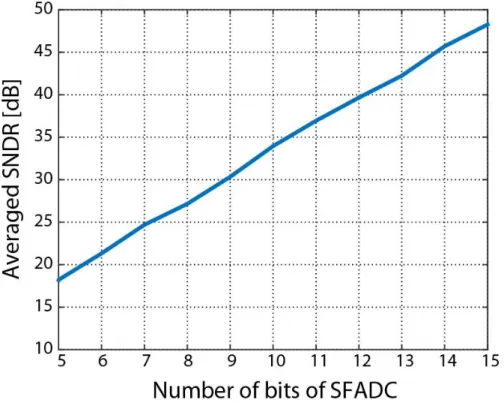
Therefore, we use Monte Carlo simulation instead of mathematical model in the case of a large number of groups to establish the relationship between SNDR and the number of comparators required. We first take samples of random variable with a given distribution, and using these values as the trip points for an ideal SFADC, and after applying a full-scale sine input, the SNDR can be calculated through 4096-point FFT. Repeating this test 100 times allows us to find the average SNDR for a given number of comparators. Fig. 3.3 reveals the relationship between SNDR and the number of bits N,

where the number of comparators is equal to 2N_{-1. It can be seen that,}

to achieve an improvement of 6dB on SNDR, the number of comparators needs to be quadrupled, which is consistent with the

conclusion in the Section 3.2.1, also the conclusions of [23,25,29-31]. Although their theoretical value of the number of comparators is

different, the conclusion that ENOB is proportional to 4N _is

consistent.

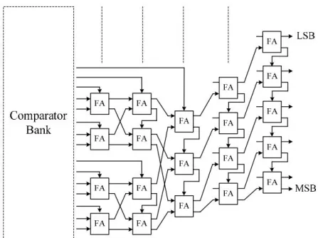
3.3 Wallace Tree Adder

The encoder counts the number of high levels output by the comparator bank and converts the result into a binary code form. The fault tolerance and speed must also be considered when designing the encoder. Working for summation of logic ‘1’, Wallace tree adder is applied to encoding of SFADC. The encoder is realized by cascading the full adder FA into a Wallace Tree structure. Fig.3.4 shows an example of 6-bits Wallace Tree encoder [32]. Assuming

that the number of full adders required for an N-bits encoder is XN.

Two N-bits encoders and N full adders forms a new (N+1)-bit encoder. Hence，         1 2 2 2 1 X ) N (for N X XN N (Eq. 3.28)

By solving the recursive sequence (Eq. 3.28), the number of full adders required for an N-bits encoder is given by



With the properties of full adder, carry input on the full adder can be equated to an addend. A full adder can therefore be regarded as a three-input adder. In accordance with weight, bits of the same weight can be connected to the common adder in the next level for a summation while the bits of different weights are separated.

Fig. 3.4: An example of 6-bit Wallace tree adder

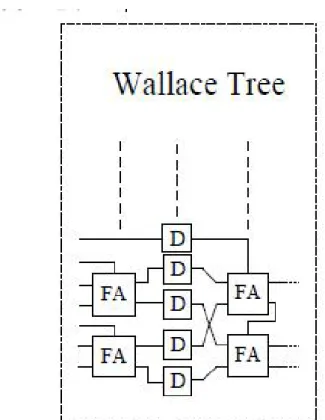
There are three advantages with this structure. Firstly, tree topology can reduce the transmission distance of digital signal, reducing the parasitic capacitance. Secondly, the structure of the Wallace tree adder doesn't concern on the order of the comparators. So Wallace tree adder structure can be flexibly designed, which makes it especially suitable for SFADC. Thirdly, the tree topology can be easily implemented in pipelined work. Inserting D-triggers to the critical path of the circuit, allows the Wallace tree adder to work at a high speed, shown as Fig. 3.5.

The maximum sample frequency is decided by adder cell delay when all of FAs are pipelined:

delay)

cell

/(adder

CHAPTER 4

Fully Synthesizable Rail-to-rail Dynamic

Comparator

Due to large-scale adoption of comparators, decreasing the power consumption of single comparators becomes an effective method to decrease the overall power consumption of SFADC. In addition, digital circuits are more profitable from scaling down compared to analog circuits. They can obtain low parasitic capacitance, supply voltage and power consumption effortlessly in this context. The synthesizable characteristic saves them from the effort for customized layouts as well. Therefore, we focus on the realization of a fully synthesizable dynamic comparator with a wide input range.

The all-digital design of comparator have been concerned. [25] proposes a dynamic comparator based on two cross-coupled 3-input NAND gates. However, the common-mode input range(CMR) is limited to a high voltage region to avoid PMOS current more robust than the NMOS current of input transistors. To address the issue of the narrow CMR, two types of methods have been proposed in previous works.

[33]–[35] introduce additional pull-down networks. When the common-mode input is a low voltage, the strong sinking current flowing via the pull-down network offsets the effect of the PMOS

current, so that low input voltages are applicable. Nevertheless, the strength of the pull-down network needs careful consideration. The strength which is too strong or too weak cannot force output to the supply rail properly. Also, the method of utilizing a pull-down network causes high power consumption due to a severe short-circuit current, which is disadvantageous for low-power design.

[36] and [37] combine the NAND-based comparator and the NOR-based comparator, utilizing the complementary features of them. When the common-mode input is close to VDD or VSS, there is always a comparator that works correctly. Through a selection mechanism, the comparator with the valid result transmits data to the final comparator output. However, the alternative mechanism may lead to incorrect output results when the CMRs of the two comparators do not intersect and the input is just falling in the gap. Besides, the robust short-circuit in their decision phase results in low power efficiency.

4.1 Review and Proposed Rail-to-rail Dynamic

Comparator

4.1.1 Review

[25] firstly proposes a dynamic comparator composed of standard cells. 3-input NAND gate is usual in the standard cell library. The manner of constructing the comparator with two NAND gates is

illustrated as Fig. 4.1. Transistors MP5, MP6, MN5 and MN6 constitute a regenerative latch. When the clock is low(reset phase), MP3 and MP4 are turned on; MN3 and MN4 are turned off. Thus output nodes Vout+ and Vout- are precharged to VDD. When the clock is switched to high(decision phase), MP3 and MP4 are turned off, thus disabling the precharge of Vout+ and Vout- . Due to the drain current difference between MN1 and MN2 induced by input voltage difference, Vout+ and Vout- drop voltage at a different speed. As Vout+ and Vout- are gradually pulled down, gate voltage on the one of PMOSs in the regenerative latch is first to reach VDD-Vth, thus enabling this PMOS to charge to corresponding output nodes. Then positive feedback effect starts and amplifies the voltage difference of output nodes. Finally, the output nodes are forced to the supply rails.

CLK CLK CLK CLK Vin+ Vin+ Vin-MP1 MP3 MP5 MP6 MP4 MP2 MN5 MN6 MN3 MN4 MN1 MN2 Vout+ Vout-(a) CLK Vin-Vin+ Vout-Vout+ (b) (NAND)×2

However, a problem arises when common-mode input is close to VSS. In this case, MP1 and MP2 are turned on, producing a stronger current than MN1 and MN2, which causes charging to output node continuously. Finally, both of the outputs are pulled up to high voltage, comparator failing to compare the two inputs. This phenomenon dramatically limits the CMR of the comparator.

4.1.2 Proposed Rail-to-rail Dynamic Comparator

In order to broaden the input range of the NAND-based comparator, we propose a block-based method to construct a dynamic comparator that is made up of two OAI211 gates(OR-AND-INVERTER). This cell is also typical in the standard cell libraries of advanced processes. Connect two OAI211 gates to construct our proposed comparator, as shown in Fig. 4.2. Different from the NAND-based comparator, MP3, MP4, MN3 and MN4 are "additional transistors" (marked in red).

CLK CLK CLK CLK Vin+ Vin+ Vin-Vout+ Vout-MP1 MP5 MP7 MP3 MP8 MP6 MP2 MP4 MN7 MN8 MN5 MN6 MN1 MN3 MN4 MN2 Vout+ Vout-CLK Vin-Vin+ Vout+ Vout-Vout+ (a) (b) (OAI211)×2

Fig. 4.2: OAI211-based Rail-to-rail Dynamic Voltage Comparator (ORDVC). (a) Schematic; (b)Symbol

MP3 and MP4 play the roles of valves controlled by the output voltage, cutting off the direct connection between the supply rail and the output nodes. The one whose gate voltage first reaches VDD in the decision phase completely blocks the current flowing from supply power to the corresponding drain. Therefore, MP3 and MP4 effectively avoid both output nodes to be pulled up to high voltages together when common-mode input is low. Since dynamic current only flows during regeneration, this structure is power-effective.

Taking advantage of the complementary idea, we further propose a variant composed of OAI211-based comparator and AOI211-based (AND-OR-INVERTER) comparator for a wider CMR, illustrated as Fig. 4.3. Somewhat different from the single comparator like OAI211-based comparator, two complementary comparators are

cross-coupled with each other, that is, they connect the gates of the additional transistors to each other’s output nodes. The complementary signal NCLK of the clock signal CLK is obtained through an inverter. When the common-mode input voltage is close to VDD, the OAI211-based portion dominates; otherwise, the AOI211-based portion dominates when the common-mode input voltage is close to VSS. Vin-Vin+ Vin-CLK CLK CLK CLK Vin+ Vin+ Vin-Vo1 Vo4 Vo2 Vo3 NCLK NCLK NCLK NCLK Vin+ Vin-Vo4 Vo1 Vo3 Vo2 MP1 MP2 MN1 MN2 MP3 MP4 MN3 MN4 (b) CLK Vo2 Vin-Vo1 Vin+ NCLK Vo3 Vin-Vo4 Vin+ (a) (OAI211)×2+(AOI211)×2

Fig. 4.3: Merged Rail-to-rail Dynamic Voltage Comparator (MRDVC). (a) Schematic; (b)Symbol

Two variants have different initial conditions when they are switched to the decision phase, which predictably brings some

differences in performances. For convenience, the OAI211-based rail-to-rail dynamic voltage comparator is called 'ORDVC' for short, and the merged version consist of the two complementary comparators is 'MRDVC'.

In terms of ORDVC in Fig. 4.2, MP3 and MP4 are cut off while MN3 and MN4 are turned on initially. On the one hand, the pull-down network is strengthened, and the pull-up network is weakened compared to a NAND-based comparator. The voltage of output nodes can swiftly meet the triggering condition of the positive feedback, which brings improvement on propagation delay. On the other hand, due to high voltage on the gates of MN3 and MN4 initially, device mismatch between MN3 and MN4 can lead to a large mismatch current. It takes a tremendous effort for the input to offset such effect, which makes comparators have a larger variation in comparator offset.

As far as MRDVC is concerned in Fig. 4.3, at the beginning of decision phase, MP1, MP2, MN3 and MN4 are turned on; on the contrary, MN1, MN2, MP3 and MP4 are cut off. At the moment, the merged comparator is shaped like an individual NAND-based comparator and NOR-based comparator. Therefore, it offers a legitimate mix of propagation delay and comparator offset variation.

4.2 Simulation

Based on the 65nm CMOS process, the prior art (Seo [33] and Aiello [36]) are replicated to compare with our proposed comparators through the simulation. Seo [33] is the most power-effective representative of the pull-down method, which adopts a power down logic for energy saving, while Aiello [36] is the representative of the complementary method. To facilitate the comparison, we use the minimum size of transistors and appropriate latches in all candidates. It is noted that for MRDVC, either Vo1, Vo2, or Vo3, Vo4 can be used as complementary outputs connected to an appropriate latch, with a little influence on the simulation result.

Under the different supply voltages, the relationship between the propagation delay and common-mode input voltage is shown in Fig.4.4 when the load is 5fF and the differential voltage is 5mV. In regard to CMR, MRDVC is the only one covering a full rail-to-rail CMR under three different supply voltages. Aiello [36] fails to output the correct results at 120 mV when the power supply is 300mV, leading to a discontinuous CMR. Seo [33] only allows the common-mode voltage higher than 1/2 VDD. ORDVC only accepts about half of the rail-to-rail CMR in the cases of VDD equal to 300mV and 600mV.

Common mode voltage [mV] 30 90 150 210 270 D el ay [n s] 0 10 20 30

40 _{Seo[33] Aiello[36]}(a) _{ORDVC MRDVC}

Common mode voltage [mV]

60 180 300 420 540 D el ay [n s] 0 0.5 1 1.5 2 _{Seo[33] Aiello[36]}(b) ORDVC MRDVC

Common mode voltage [mV]

90 270 450 630 810 D el ay [n s] 0 0.1 0.2 0.3

0.4 _{Seo[33] Aiello[36]}(c) _{ORDVC MRDVC}

Fig. 4.4: Propagation delay versus common-mode voltage under different supply voltages. (a) 300mV; (b) 600mV; (c) 900mV

In terms of propagation delay, the results suggest that ORDVC performs best. It obtains the maximum delay around the voltage close to the lower bound of CMR. MRDVC has the same trend as Aiello [36] that as the common-mode voltage goes up, the propagation delay increases first and then decreases. They both get a maximum delay at the voltages slightly below 1/2 VDD.

The relationship between the average power and common-mode voltage is obtained by providing a 5mV differential input and connecting a 5fF load. The clock frequency is set to 10MHz, 250MHz and 1GHz under the supply voltages of 300mV, 600mV and 900mV, respectively. It is reported in Fig. 4.5 that the structures based on the complementary comparators (MRDVC and Aiello [36]), always have maximum power consumption around 1/2 VDD. For the other two candidates adopting a single comparator (ORDVC and Seo [33]), they are little influenced by the common-mode voltage.

Common mode voltage [mV]

30 90 150 210 270 Po w er [n W ] 10 20 30 40

50 _{Seo[33] Aiello[36]}(a) _{ORDVC MRDVC}

Common mode voltage [mV]

60 180 300 420 540 Po w er [μ W ] 0 1 2 3

4 _{Seo[33] Aiello[36]}(b) _{ORDVC MRDVC}

Common mode voltage [mV]

90 270 450 630 810 Po w er [μ W ] 0 10 20 30

40 _{Seo[33] Aiello[36]}(c) _{ORDVC MRDVC}

Fig. 4.5: Average power versus common-mode voltage under different supply voltages. (a) 300mV (b) 600mV (c) 900mV

Fig. 4.6 shows the impact of clock frequency on power consumption when common-mode voltage is biased to 1/2 VDD and a full-scale differential input is provided. Our proposed structures play a better performance on power than the other two candidates, which are dragged down by the complex circuit structure and short-circuit current. Under the 300mV supply voltage, clock frequency does not greatly affect the power as leakage power consumption dominates. Under the 600mV and 900mV of VDD, every time the frequency is reduced by half, the power consumption of our proposed structures is also reduced by almost half, owing to the dynamic power dominating in the total power consumption. Since circuits do not always operate at the maximum clock frequency allowed by delay, our designs are attractive for power-saving in those applications with wide bandwidth. The trick to low power is that they control the dynamic power consumption caused by short-circuit current in the decision phase.

Frequency [MHz] 10 5 2.5 1.25 Po w er [n W ] 0 10 20

30 _{Seo[33] Aiello[36]}(a) _{ORDVC MRDVC}

Frequency [MHz] 250 125 62.5 31.25 Po w er [μ W ] 0.0750.15 0.3 0.6

1.2 Seo[33] Aiello[36](b) ORDVC MRDVC

Frequency [MHz] 1000 500 250 125 Po w er [μ W ] 0.450.9 1.8 3.6 7.2

14.4 Seo[33] Aiello[36](c) ORDVC MRDVC

Fig. 4.6: Average power versus clock frequency under different supply voltages. (a) 300mV; (b) 600mV; (c) 900mV

With Monte-Carlo simulation, the method in [38] is adopted to simulate the comparator offset. In our simulation setup, the maximum comparator offset variation that can be measured is around 1/3 VDD. Fig. 4.7 illustrates the impact of common-mode voltage on offset variation for the four candidates. As can be seen that all of the candidates achieve the minimum offset around 1/2 VDD. The best performers are MRDVC and Aiello [36], with a little difference between them. In the case of 300mV and 600mV supply voltage, ORDVC's offset variation is so large that it is out of the

measurable range on the entire CMR. ORDVC also performed the worst under the 0.9V supply voltage.

Common mode voltage [mV]

50 100 150 200 250 O ffs et S td D ev [m V ] 0 20 40 60

80 _{Seo[33] Aiello[36]} (a) _MRDVC

Common mode voltage [mV]

100 200 300 400 500 O ffs et S td D ev [m V ] 0 20 40 60 80 _{Seo[33] Aiello[36]} (b) _MRDVC

Common mode voltage [mV]

150 300 450 600 750 O ffs et S td D ev [m V ] 0 100 200

300 _{Seo[33] Aiello[36]} (c) _{MRDVC ORDVC}

Fig. 4.7: Comparator offset deviation versus common-mode voltage under different supply voltages. (a) 300mV; (b) 600mV; (c)

900mV

Fig. 4.8 shows the automatically generated layout through digital synthesis, demonstrating that the proposed structures are attractive for digital design. A comparison between the four dynamic voltage

derive from the simulations under the same simulation setup based on the 65nm CMOS process. Taken together, the simulation results suggest that MRDVC achieves a full rail-to-rail CMR and 4%~ 70% of power-saving(depending on clock frequency and supply voltage) compared to Seo [33] and Aiello [36], at the cost of less than 21% delay increment. ORDVC uses less than two-thirds of transistors, obtaining 45%~ 82% of power saving in contrast with the prior works. Despite more than twice the offset, ORDVC still has application scenarios, especially in stochastic flash ADC.

5.27 μm

(a)

(b)

3.9 μm

4.07 μm

3.9 μm

Fig. 4.8: Automatically generated layout based on 65nm CMOS process. (a)MRDVC with a latch; (b)ORDVC with a latch

4.3 Chapter Summary

In this chapter, we proposes a fully synthesizable rail-to-rail dynamic comparator, which can operate at a supply voltage down to 0.3V. Two variants are discussed and compared with other dynamic voltage comparators. Simulation demonstrates our proposed structures with optimum power efficiency under different supply voltages based on the 65nm CMOS process, which demonstrates that it can be competent in the SFADC with the requirements on low voltage and low power consumption.

CHAPTER 5

Linearity Enhancement Technique (LET)

5.1 Prior Works

The transfer function of the conventional SFADC has good linearity within the input range of ±1σ, so generally SFADC’ input range is between ±1σ. On the one hand, the performance of the ADC usually improves as its linear input range increases. On the other hand, the non-linear transfer function will introduce harmonics into the system, thereby reducing the SNDR of the ADC. Therefore, in order to design an good ADC, we should improve the linearity of SFADC as much as possible and broaden the input range of ADC.

Some of linearity enhancement techniques has been proposed in the prior works. A technique [23] (shown as Fig. 5.1) has been presented, which reduces this nonlinearity by changing the overall transfer function by building a two-group SFADC. Setting the references of two comparator groups to have approximately ±1σ of comparator offsets allows higher linearity to be achieved. In this method, using the exact same comparators under the same conditions but merely dividing them into two groups with different references, an 8.5-dB improvement in SNDR can be obtained and there is no additional area overhead. Linearity is improved, however,

Fig. 5.1: Two-group SFADC splitting the total number of comparators into two groups and applying an offset to each group, the shape of the transfer function can be controlled. For example, one group is given an offset of +1σ, and the other is -1σ.

The method above is further expanded in [39] (shown as Fig. 5.2). Comparators are equally divided into several comparator groups and reference voltages are equally spaced by a resistor ladder. Each group is referenced to a different reference voltage. Changing the mean (reference voltage) of comparator thresholds only shifts the transfer function along the input axis. Probability density functions (PDF) of comparator offset in each group is also shifted by the reference voltage. The overall output is obtained by summing the outputs of each group, achieving a flat top and a wide spread across the voltage range. While this method improves linearity, the input range is also greatly expanded.

Fig. 5.2: Multi-group SFADC

The prior work in [25] uses an additional hardware calibration circuit to perform piecewise linearization on the digital output, realizing a function similar to the inverse Gaussian function (shown as Fig. 5.3). The input range is extended to [-3σ,3σ]. Although this algorithm is simple, it does not calibrate the higher-order terms in the transfer function and an additional hardware overhead for the calibration is needed.

Fig. 5.3: Inverse Gaussian CDF Method

In [40], to linearize the transfer function of the SFADC, a reference voltage is added to the comparator reference terminal, shown as Fig. 5.4. The added reference voltages follow random U-quadratic distribution. In this way, the trip point of the comparators will be spread to a wider range and shaped into uniform distribution. Let f(x), g(x) and h(x) be the PDF’s of the comparators offset, U-quadratic reference signal and the resultant comparator trip points

respectively. Thus h(x) g(x) f(x)_{. In this method, the input range}

is extended to [-3σ,3σ]. However, a large number of resistors with different values are used to generate the reference voltages following a quadratic distribution.

Fig. 5.4: U-quadratic distributed reference voltages method

5.2 Our proposed Linearity Enhancement Technique

(LET)

In summary, it can be seen that the method of employing a multi-group architecture [39] can effectively extend the input range beyond [-3σ,3σ] and improve the linearity of the original transfer function to a certain extent. The above works [23,25,39,40] does not pay attention to the change of the comparator offset’s standard deviation with the common mode voltage. When the reference

voltages are different, although the distribution of the comparator offset also follows the Gaussian distribution, its shape has changed due to different standard deviation.

It will lead to a fluctuation at the top of total PDF if we simply combine these PDFs that are shifted by an equal space. Fig. 5.5 shows an example of SFADC consisting of multiply comparator groups where the number of groups is 11 and the reference voltage space is 1σ. Even though we can change comparator offset through tuning the size of transistors in the comparator against the influence of common mode voltage, it is troublesome to customize the layout of comparators for the different groups. In addition, even if a constant comparator offset’s standard deviation is guaranteed, there is still a limitation that the reference voltages should be set equally spaced.

Fig. 5.5: Total PDF when offset is not constant (Dark blue curve represents total PDF; the curves with other colors represent PDF of

the groups).

5.2.1 Description of LET

To obtain a completely linear transfer function of SFADC, the total PDF of comparator offset should have a flat top. In this work, we propose a methodology that improves the linearity of SFADC through adjusting the weight of each group’s PDF in the overall PDF. In the methodology, the comparator offset and reference voltage of the each group have more choices. Since SFADC represents probability with the yield of comparators outputting ‘one’, we can assign the number of comparators in each group to embody the weight. The value of the cumulative distribution function of the comparator offset also represents the probability that the input

probability is expressed by the proportion of the number of comparators that output 1 to the total. Thus

N N ) V P(V CDF H os in Total    (Eq. 5.1)

Where CDFtotal, NH, N are total PDF, the total number of

comparators outputting '1’ and the total number of comparators in SFADC, respectively. Similarly, i H,i i _N N CDF  _{(Eq. 5.2)}

Where CDFi, NH,i and Ni are CDF of i-th group, the number of

comparators outputting ‘1’ in the i-th group and the number of comparators in i-th group, respectively.

Since N Ni 





Combining (Eq. 5.1) to (Eq. 5.4), we can infer that i i i H,i i H,i H Total _N N_N CDF N N N N N N N CDF  





