for Transportation
and Logistics
Yasukuni NAGANUMA
∗∗, Takahito KOBAYASHI
∗∗∗and Hitoshi TSUNASHIMA
† ∗∗Nippon Kikai Hosen KK.2–1–95 Kounan, Minato-ku, Tokyo 108–0075, Japan E-mail: [email protected] ∗∗∗Graduate School of Nihon University 1–2–1 Izumi-cho, Narashino-shi, Chiba 275–8575, Japan
†Nihon University
1–2–1 Izumi-cho, Narashino-shi, Chiba 275–8575, Japan
Abstract
To enhance the safety and reliability of railway transportation, it is one of the most important tasks to check the track condition frequently and accurately. This paper de-scribes a track condition monitoring technique using car-body motions. In an inverse problem to estimate track geometry in longitudinal level from vertical car-body accel-eration and pitching rate measured by in-service vehicle, dynamic programming filter and Kalman filter were applied. Study results confirmed that proposed solutions can be used to estimate track geometry in level with desired precision.
Key words : Track Condition Monitoring, Inverse Problems, Kalman Filter, Dynamic
Programming Filter
1. Introduction
Track maintenance works based on track geometry recordings are essential to enhance the safety and comfort of railway transportation. In general, track irregularities are measured several times a month by a specially designed track geometry car. In addition, measurement devices are installed in commercial trains and the car-body acceleration has been measured frequently in order to check the track condition(1)(2)(3). The accelerometer is installed on
the car floor right above the bogie to measure signals due to track irregularity avoiding body-bending vibration. The track condition monitoring system is mainly used for the choice of area needing track tamping works for the purpose of the good riding comfort, and speed reduction is rarely ordered when the measured accelerations exceed the predetermined target values. An advantage of car-body acceleration measurement device is their simple structures, which make it easier to carry out maintenance. However, the car-body acceleration waveform is considerably different from track geometry, and the amplitude greatly depends on the vehicle speed.
If the track irregularity can be estimated from acceleration or any other signals measured in an in-service vehicle, a high frequent track condition monitoring by a portable device will be possible. Furthermore, it can be possible to check the track condition at anywhere and whenever it is needed. Based on an awareness of the issues, we have developed a method to calculate back to track geometry from measurement signals of a vehicle motion, and have proposed a method using impulse response functions(4). Followed by the previous studies,
this paper describes the result that estimated track geometry in longitudinal level from vertical acceleration and pitch-rate measured on a car-body using Dynamic Programming Filter (DPF) and Kalman Filter (KF).
2. Outline of this study
*Received 1 Apr., 2013 (No.13-0155)Track Geometry Estimation from Car-Body
Motions of Railway Vehicle*
physical systems such as vehicle dynamic simulation or digital filters can be formulated state variable estimation problem by using state-space model. The linear state space model ex-pressed by state equation (Eq. (1)) and measurement equation (Eq. (2)).
xn= Fxn−1+ Pun+ Gwn (state equation). (1)
yn = Hxn+ un (measurement equation). (2)
Where xn is the state at the number of time period n, un is an input control vector,wn is additive process noise, F is the state transition matrix, P is the input transition matrix and G is the driving matrix. In Eq. (2),ynis the measurement variables, H is the measurement matrix andunis additive measurement noise.
(b) Produce track geometry data from a random number similar to real track properties (more than wavelength 6.0 m).
(c) Calculate car-body acceleration and pitch rate above the center of the rear bogie from the track geometry data (b) with the numerical vehicle model.
(d) The Gaussian noise is applied to the car-body acceleration and the pitch rate to gener-ate measurement data.
(e) As preparations for inverse analysis, the vehicle model is simplified, and an order of the state equation is reduced.
(f) Track geometry is estimated from observation data (d) using a dynamic programming filter and a Kalman filter, respectively.
(g) Precision is confirmed by comparing estimated signal (f) with the true track geometry (b). 10 m versine signals are also compared and evaluated.
3. Numerical vehicle model and forward analysis
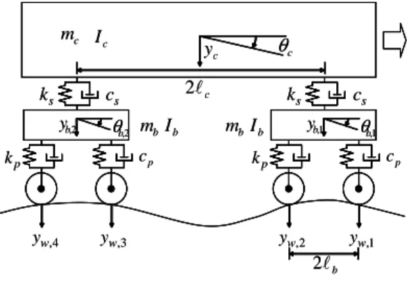
A linear vehicle model in vertical direction based on our study is shown in Fig. 1. Let
c m c θ c y c I c ℓ 2 b ℓ 2 b m s k cs p k cp 4 , w y 2 , b θ 2 , b y Ib 3 , w y yw,2 yw,1 b m s k cs p k cp 1 , b θ 1 , b y b I c m c θ c y c I c ℓ 2 b ℓ 2 b m s k cs p k cp 4 , w y 2 , b θ 2 , b y Ib 3 , w y yw,2 yw,1 b m s k cs p k cp 1 , b θ 1 , b y b I
Fig. 1 Linear vehicle model
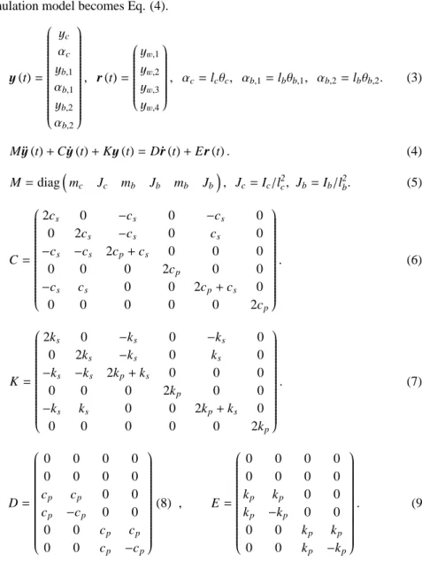
y (t) be a state variable vector and r (t) be a track geometry vector given as forced displacement
to 4 wheel sets expressed as Eq. (3), respectively. The track geometry is the average position of two rails in vertical direction. Then, the motion equation of a six-degree of freedom (DOF) To confirm the effectiveness of the inverse analysis theoretically, the following proce-dures (a)− (g) were used.
(a) The equation of vehicle motion expressed as second order differential equation is con-verted to the first order differential equation and an equation of state is obtained by discretiza-tion.
simulation model becomes Eq. (4). y (t) = yc αc yb,1 αb,1 yb,2 αb,2 , r (t) = yw,1 yw,2 yw,3 yw,4 , αc= lcθc, αb,1= lbθb,1, αb,2= lbθb,2. (3) M ¨y (t) + C ˙y (t) + Ky (t) = D˙r (t) + Er (t) . (4) C= 2cs 0 −cs 0 −cs 0 0 2cs −cs 0 cs 0 −cs −cs 2cp+ cs 0 0 0 0 0 0 2cp 0 0 −cs cs 0 0 2cp+ cs 0 0 0 0 0 0 2cp . (6) K= 2ks 0 −ks 0 −ks 0 0 2ks −ks 0 ks 0 −ks −ks 2kp+ ks 0 0 0 0 0 0 2kp 0 0 −ks ks 0 0 2kp+ ks 0 0 0 0 0 0 2kp . (7) D= 0 0 0 0 0 0 0 0 cp cp 0 0 cp −cp 0 0 0 0 cp cp 0 0 cp −cp (8) , E= 0 0 0 0 0 0 0 0 kp kp 0 0 kp −kp 0 0 0 0 kp kp 0 0 kp −kp . (9)
Define x= (y , ˙y)T be a state variable vector, the motion equation expressed as second order differential equation (Eq. (4)) is converted to the first order differential equation (Eq. (10)). ˙yy¨ = 0 I −M−1K −M−1C yy˙+ 0 0 M−1E M−1D r˙r. (10) Discretizing the Eq. (10) using numerical integration yields the following state equation:
xn+1= Fxn+ Pun. (11) xn= yn ˙ yn ∈ R12, un= rn ˙rn ∈ R8. (12)
For the discretization we used the Pade 11 method which is equivalent to the Newmark’s generalized acceleration method withβ = 1/4.
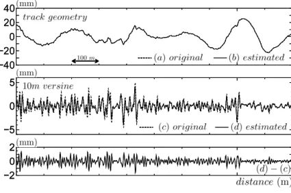
Figure 2 shows a given track geometry, calculated acceleration ¨y and pitch rate ˙θ. In the following examination, we added a Gaussian noise to calculated acceleration and pitch rate, and used these as a measurement signal. Each standard deviation of the noise is 3.0
×10−5(m/s2) and 3.0 × 10⁻⁵(rad/s).
M = diag(mc Jc mb Jb mb Jb
)
- 1 0 1 - 1 0 1 - 40 - 20 0 20 40 - 1 0 1 - 1 0 1 - 40 - 20 0 20 40
Fig. 2 Calculated acceleration and pitch rate
4. Track geometry estimation by Inverse analysis
This section analyses estimation techniques of track geometry from measured signals on the car-body. This operation is generally unstable and the calculation result greatly receives the influence of the measurement noise because it is categorized as “inverse problems” that trace the causality of stable physical phenomena in the opposite direction. Therefore, some kind of stabilization (or regularization) to reduce the influence of the noise is indispensable, and we used two techniques based on a dynamic programming filter and a Kalman filter for inverse analysis.
4.1. Simplification of numerical model for inverse analysis
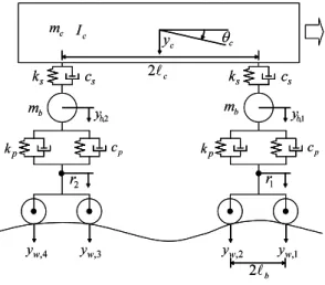
As shown in Eq. (10), an external force vector having 8 elements (track geometry at four axles and their first differential) is used in a numerical model. However, we cannot cal-culate these all 8 inputs from signals measured on the car-body, because it does not include information of the pitching motion of the bogie. In other words, we can only calculate an average geometry between front and rear axles, because input track geometry at front and rear axle are averaged by the bogie and transmitted to the vehicle body. The average geom-etry ((yw,1+ yw,2)/2(yw,3+ yw,4)/2) does not contain frequency components correspond to the wavelength of twice of the wheel base of the bogie. However, it is good enough for track management to know the average of irregularities at the front and rear wheel of the bogie, because the track irregularity is managed using 10 m-chord versine whose wavelength band of 5 m to 100 m for running stability. Therefore, the pitching of the bogie is not necessary in the vehicle model, and Fig. 1 can be reduced to 4 DOF model. A simplified model for inverse analysis is shown in Fig. 3. Four inputs can be reduced to two for inverse analysis. The following variable transformation is applied to express the simplified model. First, the average of the sum and difference of vertical displacements of the front and rear bogies, z1 and z2, are expressed respectively as follows:
z1=
yb,1+ yb,2
2 , z2=
yb,1− yb,2
2 . (13)
Assuming that r1 is the average longitudinal track level irregularity between wheels 1 and 2
and r2is that between wheels 3 and 4, then
r1= yw,1+ yw,2
2 , r2=
yw,3+ yw,4
c
m
c θ cy
cI
c ℓ 2 b ℓ 2 bm
sk
c
s p k cp 4 , w y 2 ,b y 3 , w y yw,2 yw,1 bm
sk
c
s p k cp 2 r r1 1, b y cm
c θ cy
cI
c ℓ 2 b ℓ 2 bm
sk
c
s p k cp 4 , w y 2 ,b y 3 , w y yw,2 yw,1 bm
sk
c
s p k cp 2 r r1 1, b yFig. 3 Simplified model
Further, when r+and r−are defined as follows,
r+=r1+ r2
2 , r−=
r1− r2
2 . (15)
With reduction of DOF,y (t) and r (t) in the equation of motion (Eq. (3)) are redefined as follows. y (t) = yc αc z1 z2 , r (t)= r+ r− . (16)
State vector xn and external force vector unof the discretized state equation are redefined as follows. xn= yn ˙ yn ∈ R8, u n= rn ˙rn ∈ R4. (17)
4.2. Dynamic programming filter
Trujillo and Busby pointed out that dynamic programming solution with regularization method is effective for inverse dynamic problems(5). The essence of the dynamic programming filter is to formulate an optimal control problem expressed as:
min r1:N E= N ∑ n=1 ( yn− y∗n, W ( yn− y∗n )) + (rn, Λrn). (18)
Where (•, •) denotes the inner product of two vectors and N is the number of measurements.
W is the weighting matrix that provide the flexibility of weighting the measurement. Usually
W is the identity matrix. Λ is called Tikhonov regularization parameter which reduces the
influence of the noise and controls the amplitude of input rn. When theΛ value is small, the Tikhonov regularization becomes close to the unregularized least squares solution and carries on its instability. By contrast, when theΛ value is large, the Tikhonov regularization merely minimizes the input rnand separates from the original subject. The symboly∗nis the measurement data andynis the state variable corresponding to the measurements. The symbol
yncan be related to xnby the measurement equation defined as:
yn= Hxn. (19)
are obtained respectively. The first step is to conduct backward sweep as described below. D−1n−1= D−1n − 2PTYnLnYnTP, (20) Kn−1 = Kn+ ( 2KnPTY LnYnTP− YnLnYnTP ) Dn−1, (21) Yn−1 = FT ( I− 2KnPT ) Yn, (22) Ln−1 = Ln+ LnYnT2PDn−1PTYnLn, (23) sn−1 = −2HTWyn−1+ F T(I− 2K nPT ) sn. (24)
The above equations were processed under the following initial conditions at the calculation starting point, n= N. D−1N = 2Λ + 2PTHTW HP, (25) KN = HTW HPDN, (26) YN = FTHT, (27) LN = −W + WH2PDNPTHTW, (28) sN = −2HTWyN. (29)
During the backward sweep process, all vectors DnPTsn sn and matrices KTnF should be stored. For the forward sweep, the following Eq. (30) and(31) are calculated from n= 1.
un = −Dn+1PTsn+1− 2KTF xn. (30)
xn+1= Fxn+ Pun. (31)
As preparations for inverse analysis, Eq. (10) is transformed and track geometry vector should be included in the state variable.
yy˙¨ ˙r = −M0−1K −MI−1C M−10E 0 0 0 yy˙ r + M−10D I ˙r (32)
This operation decrease elements of the external force vector un to 2 from 4. During the forward sweep, the quantity ˙rnis calculated as external force. And the quantity rnis given as elements of the state variable vector rn = (r+, r−)T by solving an Eq. (31) at the same time. The mean track geometry at front and rear position is calculated by;
yw,1+ yw,2
2 = r++ r−,
yw,3+ yw,4
2 = r+− r−. (33)
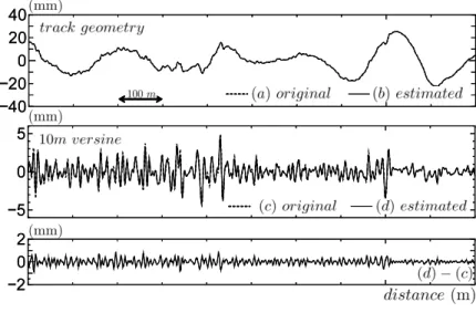
The result of inverse analysis using the dynamic programming filter is shown in Fig. 4 and 5. Figure 4 is the results when the Tikhonov regularization parameterΛ is zero. The estimated track geometry is very noisy because the solution with no regularization becomes a simple least squares estimation with its extreme sensitivity to noise on the measurement data. Figure 5 shows the results whenΛ = 1.0 × 10⁻⁵. This is the most suitable value that was found by changingΛ. The estimation is very smooth and consistent with the true track geometry, demonstrating that the dynamic programming filter with regularization is effective for the inverse analysis with acceptable accuracy. The maximum estimated error of the 10 m versine signal was approximately 1.5 mm. There exist some methods that can be used to estimate the optimum value ofΛ in practical use. They are called generalized cross validation and L-curve method.
As described above, the dynamic programming filter is mathematically simple and is easy to implement. It is advantageous in that it is independent of the number of measurements. On the other hand, the dynamic programming filter is not suitable for online real-time operation because it requires both backward and forward sweep calculation steps.
- 40 - 20 0 20 40 - 5 0 5 - 2 0 2 - 40 - 20 0 20 40 - 5 0 5 - 2 0 2
Fig. 4 Estimated track geometry by DP filter (Λ = 0.0)
−5 0 5 −2 0 2 −40 −20 0 20 40 −5 0 5 −2 0 2 −40 −20 0 20 40
Fig. 5 Estimated track geometry by DP filter (Λ = 1.0 × 10⁻⁵)
4.3. Kalman filter
A Kalman filter is a well-known algorism that estimates unknown state of the system from measurement signal containing noise. It is suitable for a real-time estimation. A proce-dure of the Kalman filter with input is shown below.
xn|n−1 = Fnxn−1|n−1+ Pnun, (34) Vn|n−1= FnVn−1|n−1FnT+ GnQnGTn, (35) Kn = Vn|n−1HnT ( HnVn|n−1HnT+ Rn )−1 , (36) xn|n = xn|n−1+ Kn (y n− Hnxn|n−1 ), (37) Vn|n = (I − KnHn) Vn|n−1. (38) xn+1 =F Pxn + I 0wn . (39)
In the procedure of the Kalman filter, the external input unin the state equation is treated as known determinate signal. The authors showed that the Kalman filter is applicable for inverse analysis if the track irregularity is expressed in a random-walk model(4). Based on similar ideas, we incorporate a random walk model (un+1 = un+ en) in Eq. (32). Specifically, the external force vector (first differential of the track geometry) is included in the state variable vector as Eq. (39).
In this study, the symbolΩ denotes the identity matrix, and the process noise wn is set to 0. The measurement equation is shown in Eq. (40).
dn= ( H 0) xn un + un. (40)
The inverse analysis of the track geometry using the Kalman filter is enabled based on Eqs. (38) and (39). In the step of the calculation, the track geometry is estimated as the state variable vector sequentially and stably.
The result of inverse analysis using the Kalman filter is shown in Fig. 6 and 7. The same simulated noise (the standard deviation of measurement noise (un) was 3.0 × 10⁻⁵(m/s2) and
3.0 × 10⁻⁵(rad/s) gives a high frequency noise in a calculation result (Fig. 6).
−2 0 2 −40 −20 0 20 40 −5 0 5 −2 0 2 −40 −20 0 20 40 −5 0 5
Fig. 6 Estimated track geometry by Kalman filter (un: 3.0 × 10⁻⁵(m/s2) and
3.0 × 10⁻⁵(rad/s))
Therefore after assuming these 0.3 (m/s2) and 0.3 (rad/s), a good result was provided as seen in Fig. 7. The difference between estimated and the true track geometry was less than 1.0 mm, confirming that the Kalman filter is effective for track condition monitoring.
−40 −20 0 20 40 −5 0 5 −2 0 2 −40 −20 0 20 40 −5 0 5 −2 0 2
Fig. 7 Estimated track geometry by Kalman filter (un: 0.3 (m/s2) and 0.3 (rad/s))
5. Conclusion and future topics
filter to model-based track condition monitoring by using signals easily measured on a vehicle body. The research study has yielded the following conclusions:
• In the inverse analysis, 8 inputs (track geometry at 4 axles and their differential
sig-nals) are not able to calculate from 2 measurements (acceleration and pitch rate) measured on vehicle body. In consideration of practical track management, we solved this problem by simplifying a numerical model.
• The dynamic programming filter with regularization was used to estimate vertical track
geometry from car-body observations. Estimated error of the 10 m versine is approximately 1.5 mm. It can be concluded that this filter can be used to calculate back the track geometry with accuracy sufficient for track condition monitoring. It is not suitable for online real-time operation because it requires both backward and forward sweep calculation steps.
• The Kalman filter became able to apply to inverse analysis by expressing track
geom-etry in a random walk model, and having incorporated the model in an equation of state. As a result of calculation, it was confirmed that the Kalman filter could estimate 10 m versine irregularity with an error within 1.0 mm from the measurement signals including the noise. The application to a track condition monitoring device is expected because the Kalman filter is suitable for a real-time processing.
It is notable that both the dynamic programming filter and the Kalman filter can support a change of the vehicle speed. Confirmation of the effectiveness using true measurement signals and the estimate of other track geometry including cross level are tasks in the near future. We determined the value of the regularization parameter, dispersion of the system and observation noise by trial and error in this study. It is one of the important tasks to find the guideline for parameter selection in these inverse problems.
References
( 1 ) H. Tsunashima, Y. Naganuma, A. Matsumoto, T. Mizuma and H. Mori, “Condition monitoring of railway track using in-service vehicle, Reliability and safety in railway”,
InTech, Chapter 12 (2012) .
( 2 ) H. Tsunashima, Y. Naganuma, A. Matsumoto, T. Mizuma and H. Mori, “Japanese rail-way condition monitoring of tracks using in-service vehicle”, Proceedings of RCM 2011 (2011).
( 3 ) Y. Naganuma, M. Kobayashi and T. Okumura, “Inertial measurement processing tech-niques for track condition monitoring on shinkansen commercial trains”, Journal of
Mechanical Systems for Transportation and Logistics 3(1) (2010).
( 4 ) T. Kobayashi, Y. Naganuma and H. Tsunashima, “Condition Monitoring of Shinkansen Tracks Based on Vehicle Model”, Proceedings of STECH 2012 (2012).
( 5 ) Trujillo, D.M. and Busby,H.R., “Practical Inverse Analysis in Engineering”, CRC
Press, New York (1997).
( 6 ) Y. Naganuma and Y. Sato, “Track state control with use of real time digital data pro-cessing”, International Journal of Heavy Vehicle Systems 2000, Vol. 7, No. 1, pp. 82-95 (2000).
( 7 ) Y. Naganuma and A. Yoshimura, “Reconstruction and estimation of railway track ge-ometry using regularization methods”, Proceedings of IAVSD 2009 (2009).
( 8 ) Y. Naganuma, T. Kobayashi and H. Tsunashima, “Study on track geometry estimation from car-body acceleration in Japanese”, Proceedings of J-RAIL 2012 (2012).