グラフの
Tutte
多項式計算システム
$=$
A
Systemfor
Computing theTutte Polynomial of
a
Graph今井浩 関根京子
Hiroshi IMAI Kyoko SEKINE
東京大学大学院理学系研究科
〒 113-0033東京都文京区本郷7-3-1
Abstract: The invariant polynomials of discrete systems such
as
graphs, matroids,hyper-plane arrangements, and simplicial complexes, have been theoretically investigated actively
in recent years. These invariants include the Tutte polynomial of a graph and a matroid,
the chromatic polynomial ofagraph, the network reliability ofanetwork, the Jones
polyno-mial of a link, the percolation function of a grid, etc. The computational complexity issues
of computing these invariants have been studied and most of them are shown to be
#P-complete. But, these complexity results do not imply that we cannot solve agiven instance
of moderate size. To meet large demand of computing these invariants in practice, there
have been proposed a framework of computing the invariants by using the binary decision
diagrams (BDD for short). This provides mildly exponential algorithms which are useful
to solve moderate-size practical problems. This paper surveys the BDD-based approach to
computing theinvariants, and describe computational resutls of the
sy.stem
which has beendeveloped for practicaluse.
Keywords: Tutte polynomial, graph, matroid, BDD, $\#\mathrm{P}$-complete, mildly exponential
al-gorithm
1
Introduction
This paper concerns computing the invariant
polynomial of discrete systems, specifically the
Tutte polynomials of graphs and matroids and
their variants. The theory$\dot{\mathrm{o}}\mathrm{f}$
theseinvariant
poly-nomials was originated around the
b’e
ginning ofthis century, and it has been extended to
vari-ous fieldsconnected with discrete systems $[3, 26]$
.
$\mathrm{C}\mathrm{o}\mathrm{m}$putationa $’$
l aspectsof these invariant
polyno-mials have
been.
a hot topic in these ten years,because its computation is very useful in a
vari-ety of fields [26]. This computation problem is
$\#\mathrm{P}$-complete in general. Recently, the binary
de-cision diagram, BDD, has been used to solve this
combinatorialproblem efficiently [17]. This paper
first describes the theory of these invariant
poly-nomials briefly, and surveys the
comput.
$\cdot$
a.t.ional
approach in detail.
The Tutte$\mathrm{p}\mathrm{o}.$
l.yno.m
ial$0,\mathrm{f}$: agraph is one of
fun-damental invariants in graph theory, which was
proposed by Tutte [23]. As for invariant
poly-nomials of a graph, the chromatic polynomial,
which denotes the number of vertex colorings such
that notwo adjacentvertices have thesamecolor,
seems more popular. This might be because the
well-known 4-colortheorem of a planar graph. In
fact,the chromatic polynomialwasoriginally
con-sidered to tackle this problem around 1912 (see
$[25, 26])$
.
TheTutte polynomialcan be naturallydefined
for matroids. The Tutte polynomial $T(M;x, y)$
ofamatroid $M$is atwo-variable polynomial of$x$
and $y$
.
This polynomial has many combinatorialmeanings. For example, the following invariant
polynomial- of discrete systems are $\mathrm{s}\mathrm{p}\mathrm{e}\mathrm{c}..\mathrm{i}.\mathrm{a}.1$
cases
of the Tutte polynomial.
$\bullet$ the chromatic
poly.n.omial
and flowpolyno-$..\mathrm{m}\mathrm{i}\mathrm{a}.1\backslash .$ . of
agraph
$\bullet$ the network reliability of
a
network$\bullet$ the partition function of
an
Ising model anda $Q$-state Potts model
$\bullet$ theJones polynomial ofan alternating link
$\bullet$ the $\mathrm{w}\mathrm{e}\mathrm{i}\mathrm{g}\mathrm{h}\mathrm{t}^{\backslash }$
enumerator of a linear code
over
$GF(q)$
$\bullet$ the shelling polynomial and the
characteristic
polynomial ofamatroid complex
Also, values of the Tutte polynomial$T(M;x, y)$of
a matroid $M$ with two variables $x$ and $y$ at some
typical points $(x, y)$ havethe following meanings.
$\bullet$ $T(M;1,1)$ is the number of bases of$M$
(span-ning trees in the case ofagraph)
$\bullet$ $T(M;2,1)$ counts the number of independent
sets of$M$ (forests in the caseofa graph)
$\bullet$ $T(M;1,2)$ counts the number of spanning
sets
$\bullet$ $T(M;2,\mathrm{o})$ is the number of cells of a
cen-tral arrangement of
a
linear matroid on$\mathrm{r}\mathrm{e}\mathrm{a}\mathrm{I}\mathrm{s}$and is the number of acyclic orientations of
a graph
For moredetails, see $[3, 26]$
.
The problem of computing the Tutte
polyno-mial, $T(G;x,y)$, of a graph $G$ is $\#\mathrm{P}$-complete in
general, except in
some
special cases such as thenumber $T(G;1,1)$ of spanning trees. For
exam-ple, when $x=2$ and $y=1$, it gives the
num-ber of forests, and this computation becomes
#P-hard. That is, in most cases, it is in a
complex-ity class at least as intractable as NP and
there-fore
seems
unlikely to have a polynomial timesolution. Recently, Alon, Frieze and Welsh [1]
developed fully polynomial time randomized
ap-proximation schemes for approximating thevalue
of the Tutte polynomial for any dense graph $G$,
whenever$x,y\geq 1$
.
This resultwas
extended toa
general graph by Karger [10]. Hence thisis
espe-cially useful for calculating the approximate
val-ues
of the Tutte polynomials which have specialmeanings such as the number offorests.
On the other hand, the exact computation of
the Tutte polynomial still remains a challenging
problem. Although exponential time would be
inevitableforthe exact computation inview of the
$\#\mathrm{P}$-completeness, reducing the exponent would
enableusto solvemoderate-sizeproblems. Mildly
exponentialalgorithms
are
practically important.There has been proposed a BDD-based
ap-proachto tackle thesehardproblem. The binary
decision diagram, BDD for short, has been used
in VLSI CAD formanipulating Booleanfunctions
in an efficientway [2]. A general package of BDD
has been developed. It is powerful enough
com-pared with other methods of handling Boolean
functions, but such a general approach has
ap-parent limitation to the
ntte
polynomialcom-putation. Sekine and Imai [17] propose a
top-down construction algorithm of the BDD
repre-senting all spanning trees of a graph, and then
Imai, Iwata, Sekine and Yoshida [9] the BDD of
bases ofa binary and ternary matroid. This
ap-proach can be generalized to solve related
prob-lems, such
as
computing the Jones polynomial ofa link, and thenumber of ideals of a partially
or-dered set. Such arelation between the BDD and
the Tutte polynomial computation has been
rec-ognized in a series ofpapers [6, 17, 20, 21], from
which interesting insights can be obtained from
both sides.
The paper proceeds as follows. The section 2
introduces the Tutte polynomial ofamatroid, and
mentions
a fundamental
result forcomputing theTutte polynomial ofagraph. Then the section 3
describesthe BDD-based paradigm for this
com-putationfor graphs. The time and space
complex-ities ofthe algorithms are analyzed for complete
graphs and planar graphs. As a specific example
how the computation of
some
special case of theTutte polynomial is interesting, the network
reli-abilitycomputation is discussed in thesection 4,
together with computational results of the real
system of comuting the Tutte polynomial.
2
Tutte Polynomial:
Definitions
and
Naive
Algorithm
The Tutte polynomial is defined for a general
ma-troid$M$, but
wee
willbe mainly concerned withalinear matroid $M$ onafinite set $E$
.
Formatroids,see
[3, 13, 25]. The most typical linear matroid isthat
over
the reals. Given a set $E$ of $m$ vectors$a_{1},$$a_{2},$$\ldots,$ $a_{m}$ in $\mathrm{R}^{n}$, linear independenceamong
vectors in $E$
.
The rank function $\rho:2^{E}arrow \mathrm{Z}$ of$M(E)$ is defined by
$\rho(S)=\dim(\{a_{i}|a_{i}\in S\})$ $(S\subseteq E)$
.
where the righthand is the dimension of a space
spanned by $a_{i}(a_{i}\in S)$. The linear matroid
$M(E)$of vectors$a_{i}\in E$canbe regardedasthat of
the arrangement of hyperplanes $h_{i}=\{x|a_{i}\cdot x=$
$0\}$ $(i=1, \ldots , m)$ in the dual $\mathrm{R}^{n}$
.
The Tutte polynomial$T(M;x, y)$ of matroid$M$
on $E$ is a two-variable polynomialof$x$ and $y$
.
Bythe rank function $\rho$, it is defined by
$T(M;x, y)=S \subseteq\sum(_{X}-1)\rho(E)-\rho(A)(y-1)^{1}Es|-\rho(S)$
.
The original definition of the Tutte polynomial
by Tutte is expressed as the summation over all
bases of a matroid. To describe this, we need
more definitions. Let $B$ be abaseof matroid $M$
.
For $e\in E-B$, a minimal dependent set of $B\cup$
$\{e\}$, including $e$, is uniquelydetermined, which is
called thefundamental circuitof$e$with respect to
$B$
.
For $e\in B,${
$d\in E|(B-\{e\})\cup\{e’\}$isabase}
is called thefundamentalcutset of$e$ with respect
to$B$
.
Given anordering $e_{1},$ $e_{2},$$\ldots.e_{m}$of elementsof$E,$ $e_{i}\in E-B$ is called externally active if its
fundamental circuit with respect to $B$ consistsof
$e_{j}$ with$j\leq\dot{i}$
.
$e_{i}\in B$ is called internallyactive ifits fundamental cutset with respect to $B$ consists
of$e_{j}$ with$j\leq i$
.
Then,for$B$, theexternalactivity
$r(B)$ is the number of external active elements,
and the internal activity $s(B)$ is the number of
internal active elements. Then, for this ordering,
the ntte polynomial is given by
$\tau(M;x, y)=:\mathrm{a}S\sum_{B\mathrm{b}\mathrm{e}\mathrm{s}\mathrm{o}\mathrm{f}M}x^{r})(B)_{y^{S}}(B$
.
The Tutte polynomial of matroid $M$ has many
meanings. For example, $T(M;1,1)$ is the number
of bases of$M$, since it counts the number of
sub-sets $S$ with $|S|=\rho(S)=\rho(E)$. $T(M;2,1)$ the
number of independent sets of$M$, and$T(M;1,2)$
the number of spanning sets of $M$ (see [3, 26]).
With the arrangement of hyperplanes such that
all the hyperplanes pass the origin, a linear
ma-troid $M$
over
the reals is associated ina
straight-forward way. An arrangement is central if their
hyperplanes have non-empty
common
intersec-tion, andourarrangement is central. In this case,
$T(M;2,0)$ givesthe number of regions of this cen-tral arrangement.
When the
ntte
[23] introducedthe Tuttepoly-nomial, he also showed it has the recursive
for-mula. This formula holds for matroids, but from
here in thissection wedescribe thecaseofagraph
to state
a
specific complexity ofsomefundamen-tal algorithm.
Theorem 1 For $e\in E$, the Tutte polynomial
$T(G;x, y)$ is expanded as
follows:
$\{$
$xT(G/e;x, y)$ $e$: coloop
$yT(G\backslash e;X, y)$ $e:l_{oO}p$
$T(G\backslash e;x, y)+T(G/e;x, y)$ otherwise
Here, foranedge$e$ in$E$, wedenote by$G\backslash e$ the
graph obtained bydeleting $e$from $G$, and by$G/e$
the graph obtained by contracting $e$ from $G$
.
Aloop is an edge connecting the same vertex, and
a coloop is an edge whose removal decreases the
rank of the graph by 1. If$G$ is a connected graph
a coloop is an edge of $G$ whose removal
discon-nects $G$
.
By definition, the Tutte polynomial ofa loop is $y$ and that of a coloop is $x$
.
The Tuttepolynomial of a graph with no edge is 1. Note
that the deletion, contraction, loop, and coloop
are all defined for matroids.
By applying the above formula recursively for
anedgechosenbyany order we canalso compute
the Tutte polynomial. This computation process
corresponds to top-down fashion foranexpansion
tree (Fig. 1). The root corresponds to the graph
$G$, and each parent has at most two children. For
each path from the root to a leaf in the
expan-siontree, when acoloop is contractedor aloop is
deleted, $x$
or
$y$ is multiplied, respectively. Thenthe sum of the leaves is the Tutte polynomial of
agiven graph $G$
.
Here, for each path from the root to a leafin
the expansion tree, a set ofcontracted edges
cor-responds to a spanning tree of $G$one-to-one. For
example, the most left path in Fig. 1 corresponds
to the spanning tree $\{e_{1}, e_{2}, e_{3}\}$
.
Then thenum-ber of leaves equals the numnum-ber of spanningtrees.
The depth of the expansion tree is $|E|$, Since the
depth of the expansion tree is $|E|$
,
by using thisexpansion tree in a clever way we obtain the
fol-lowing bound. For more details of existing
level $0$ 1 2 3 4 5 $y^{3}!$
.
$y^{2}.\cdot$.
$xy|$ $y^{2}|$:
$xy|y:$
.
$x|$ $x^{2}|$ $y^{2}:.x.y:y:$.
$x|$ $x^{2}|$ $x.y$:
$x^{2}|$ $x^{3}|$6
Figure 1: Expansion tree for complete graph $K_{4}$
Theorem 2 $Us\dot{i}ng$ the $recurS\dot{i}ve$ formula, the
Tutte polynomial
of
a graph $G=(V, E)$ can becomputed in $O(|E|\tau(c;1,1))$ time.
3
Tutte
Polynomial:
BDD-based
Algorithms
In this section, a BDD-based algorithm for
com-puting the Tutte polynomial of a graph, which
does not taketimeproportional to the number of
spanning trees.
For a given graph $G$
,
order the edges$e_{1},$ $e_{2},$$\ldots,$$e_{m}(m=|E|)$
.
Suppose we apply therecursive formula in the order of$e_{1},$ $e_{2},$$\ldots,$ $e_{m}$ in
a top-down fashion as in the expansion tree
de-scribed in the previous section. Agraph obtained
from$G$ by deletions $\mathrm{a}\mathrm{n}\mathrm{d}/\mathrm{o}\mathrm{r}$contractions of edges
is called
a
minorof $G$.
Nodes in the i-th level inthe expansion treecorrespondtominorsof$G$with
the edge set $\{e_{i+1}, e_{i+}2, \ldots, e_{m}\}$ (the O-th level is
the root). Since the
ntte
polynomial is anin-variant for isomorphic graphs,
we
may representisomorphic minors among them by
one
of thesemembers. However, for given two graphs, there
is no efficient algorithm to decide whether they
are isomorphic or not and finding all isomorphic
minors may be difficult.
The isomorphism between two graphs whose
edges have an identity map can be determined
in linear time. For this reason,
we
may restrictourselves just to finding isomorphic minorswhose
corresponding edges have the same order in the
originalgraph $G$
.
By merging the isomorphicmi-nors
with thesame
edge ordering, the expansiontree becomes an acyclic graph (anedgeis directed
from a parent to achild). See an example of the
complete graph $K_{4}$ in Fig.2. This acyclic graph
has asingle
source
(theoriginal graph$G$) and them-th level may be regarded as a single sink.
Rigorously, the acyclic graph representing the
computation process can be constructed
as
thefollowing algorithm, where$S_{i}$ is $\mathrm{t}$
.he
set ofminorsin the i-th level.
So
$:=\{G\}$;for $i:=1$ to $m$ do
begin
$S_{i}:=\emptyset$;
for each minor $\overline{G}$
in $S_{i-1}$ do
$vsvv_{1}2$ $\mathrm{c}\mathrm{o}\mathrm{n}\mathrm{t}\mathrm{r}\mathrm{a}\mathrm{c}/\mathrm{t}$ $.\sim_{\mathrm{c}_{\mathrm{c}}}\sim$ delete $.\sim$
.
end end end;Via the above computation process, the Tutte
polynomial can be computed as follows. The
next algorithm shows the Tutte polynomial
can
be computed by top-down fashion and need not
by bottom-up fashion. Here atwo-variable
poly-nomial $t(v;x, y)$ is associated with each minor $v$
in the computation process.
$(y+2)(\mathrm{o}_{3}+x+2y)v_{2}vv4v2v_{3}\Leftrightarrow^{v}4u_{6}\mathrm{L}\mathfrak{Z}_{2}vv4(x+2v_{3}\Delta)v_{4}$
....
$\mathit{1}_{6}^{v_{2}}5vsv4$$.\backslash .$
.
$|$$\frac{\backslash \backslash \backslash \backslash \sim\backslash \backslash \backslash \backslash \backslash \backslash \backslash \backslash }{}$
$(2x+2+3y+y)2$ $v_{3}v_{4}\mathrm{Q}$
$(x^{2}+3x+2+2y)$ $\underline{v_{3}}v_{4}$
$\backslash \backslash \mathrm{c}\mathrm{c}$
/
$x^{3}+3x^{2}+2X+4xy+2y+3y^{2}+y^{3}$
Figure 2: Computationprocess of$T(K_{4;y}x,)$
begin
if$e_{i}$ is a loop in
$\overline{G}$
then
child$(\overline{G}):=\{\overline{G}\backslash ei\}$
else if$e_{i}$ is acoloop in
$\overline{G}$
then
child$(\overline{c}):=\{\overline{c}/e_{i}\}$
else (comment: $e_{i}$ is neither a loop nor
a coloop) child$(\underline{\overline{c}}):=\{\overline{G}\backslash e_{i},\underline{\overline{c}}/e_{i}\}$;
for each minor $G_{e_{i}}$ in child$(G)$ do
begin
check if there is anisomorphic graph
with the
same
edgeordering in Si;if there is suchanisomorphic graph
$\hat{G}$in
$S_{i}$then construct anedge from
thenode representing$\overline{G}$tothe node
representing $\hat{G};-$
otherwise, add $G_{e_{i}}$ to $S_{i}$ and
con-struct anedge from the node
repre-senting $\overline{G}$
to the node of$\overline{G}_{e_{i}}$;
$t(\mathrm{s}\mathrm{o}\mathrm{u}\mathrm{r}\mathrm{C}\mathrm{e};x, y):=1$;
for $i:=1$ to $m$ do
begin
for all nodes $u$ in $S_{i}$ do $t(u;x, y):=0$;
for each node $v$ in $S_{i-1}$ do
begin
if$v$ has two children $u,$ $w$ then
begin
$t(u;x, y):=t(u;x, y)+t(v;x, y)$ ; $t(w;x, y):=t(w;x, y)+t(v;x, y)$
end
else (comment: $v$ has only one child $u$)
if$e_{i}$ is a loop then
$t(u;x,y):=t(u;x, y)+yt(v;x, y)$
else (comment: $e_{i}$ is acoloop)
$t(u;x, y):=t(u;x, y)+xt(v;x, y)$ ;
end end;
$t(\mathrm{s}\mathrm{i}\mathrm{n}\mathrm{k};x,y)$is $T(G;x, y)$
.
3.1
Decision of
Isomorphic MinorsThe size of the computation process is defined
as the number of minors which
occur
incomput-ing the Tutte polynomial by the algorithm. The
width is definedasthe maximum among the
num-bersof minors of the computation process at each
level. The depth of the computationprocessis the
number of edges. Hence the width of the compu-tation process is relevant.
Suppose that $E_{i}=\{e_{1}, e_{2}, \ldots, e_{i}\},$ and $\overline{E_{i}}=$
$\{e_{i+}1, e_{i+2}, \ldots , e_{m}\}$
.
Then theminors of$G$in thei-th level have the edge set$\overline{E_{i}}$
.
For$\dot{i}=1-,$$\ldots$,$m$,
define the $\dot{i}$-th level elimination front $V_{i}$ to be a
vertex subset consisting of vertices $v$ such that $v$
is incident to
some
edges in $E_{\mathrm{i}}$ and someedges in$\overline{E_{i}}$
.
By the edges contracted in this$\underline{\mathrm{p}}\mathrm{r}\mathrm{o}\mathrm{C}\mathrm{e}\mathrm{S}\mathrm{S}$, we
two vertices are in the same equivalence class if and only if, in the process of obtaining the minor,
they are unified into one vertex by the
contrac-tions. Then consider a partition of $\overline{V_{i}}$ into the
equivalence classes by this relation. We call this
partition the$\dot{i}$
-th level elimination partition of the
minor. For example, in Fig. 2the third level
elim-ination front is$\{v_{2}, v_{3}, v_{4}\}$
,
sinceallincidentedgesof $v_{1}$
are
contractedor
deleted. When $e_{1}$ and $e_{2}$are
contracted and $e_{3}$ is deleted, $v_{2}$ and $v_{3}$ areunified into one vertex. In this case, the
elimina-tionpartition of this minor is $\{\{v_{2}, v_{3}\}, \{v_{4}\}\}$. By
using these definitions, we can derive the
follow-ing.
Theorem 3 Let$H_{1}$ and$H_{2}$ be two minors
of
$G$with the same edge set $\overline{E_{i}}$
.
$H_{1}$ and $H_{2}$ areiso-morphic with the
same
edge orderingif
and onlyif
their i-th level elimination partitions areiden-tical.
This theorem
can
be used not only to checkthe isomorphism
more
easily but also to analyzethe size of thecomputationprocess. Furthermore,
checking whether twopartitions are identical can
be done very easily.
The Tutte polynomial is an invariant for
2-isomorphic graphs which is related to
isomor-phism of matroids. If two graphs $G_{1}$ and $G_{2}$
are isomorphic then they are also 2-isomorphic,
although
we
can merge only isomorphic minorswith thesameedge ordering by using Theorem3.
For agiven connected graph if the edge
order-ing hasaconnectedness property, all 2-isomorphic
minors with the same edge ordering are
isomor-phic minors with the same edge ordering. Here,
the edge ordering is assumed to have a
connect-edness property if for $\dot{i}=1,$ $\ldots$,$m$, all subgraphs
of $G$on$\overline{E_{i}}$
are
connected.Theorem 4 Suppose that the edge ordering has
the connectedness property
for
a given connectedgraph G. Let $G_{1}$ and $G_{2}$ be two minors
of
$G$ onthe same edge set $\overline{E_{i}}$
.
Then $G_{1}$ and $G_{2}$ are2-isomorphic with the
same
edge ordering.if
andonly $\dot{i}fG_{1}$ and$G_{2}$ are isomorphic with the same
edge ordering.
For proofs of these theorems, see [19].
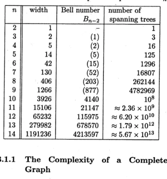
Table 1: The sizeof$\mathrm{c}\mathrm{o}\mathrm{m}.\mathrm{p}..\mathrm{u}\mathrm{t}\mathrm{a}\mathrm{t}\mathrm{i}_{\mathrm{o}\mathrm{n}}$process of$K_{n}$
3.1.1 The Complexity of a Complete
Graph
We consider the size of the computation process
of a complete graph $K_{n}$ of $n$ vertices, since it is
the upper bound for the other simple connected
graphs.
For the complete graph $K_{n}$ of$n$ vertices, order
the vertices from 1 to $n$
.
Then, represent eachedge by a tuple $(u, v)$ where $u$ and $v$ are
num-bers attached to their endpoints and $u<v$, and
order edges in the increasing lexicographic order
of $(u, v)$
.
This ordering is called a canonical edgeordering of
a
complete graph.Let $L(G_{\dot{i}},)$ be the number ofminors in the i-th
level of the computation process for the
canoni-cal edge ordering. Since each parent has at most
two children, $L(G,\dot{i})\leq 2^{i}$. Moreprecisely, for the
complete graph $K_{n}$, the following theorem holds.
Here the Bell number $B_{n}$ is thenumber of
Parti-tionsof a set of$n$ elements.
Theorem 5 $L(K_{n},\dot{i})=2^{O(i)}$
for
$\dot{i}\leq 2n-3$, and$L(K_{n}, i)\leq B_{j}$
for
$2n-3<i$.
Corollary 1 For $n\geq 10$, the width
of
thecom-putationprocess
of
$K_{n}$for
the canonical edgeor-dering is bounded by$B_{n-2}$
This bound is not so tight. Table 1 gives the
width and the size of thecomputation process of
$K_{n}$ upto $n=14$
.
It also shows thewidth can bebounded by $B_{n-2}$ for $n\geq 10$ and much smaller
Theorem 6 For any simple connected graph $G$
with$n$ vertices, there exists an edge ordering such
that the size
of
the computation processof
$G$ isless than or equal to the size
of
the computationprocess
of
the complete graph $K_{n}$ with respect tothe canonical edge ordering.
Note that, in computing the Tutte polynomial
of agraph with $n$ vertices $(n\geq 10)$ via the
com-putation process, the space complexity is also
boundedbythe width of thecomputation process
and hence by $B_{n-2}$
.
This is another advantage ofthis algorithm.
3.1.2 The Complexity ofa Planar Graph
Next, we will see that the proposed algorithm
solves the problem of computing the Tutte
poly-nomial ofa planar graph, which itself is still
#P-hard, very efficiently.
First, to examine its efficiency for a planar
graph, we will consider its computational
com-plexity of a lattice graph. The (square) lattice
graph $L_{m,n}$ is a graph which has $m\cross n$ vertices
located at the points $(x, y)$ of the 2-dimensional
grid with edges joining neighbours on the grid.
The lattice graph is extremely important for a
number of problems in statistical physics.
For a$k\cross k$ lattice graph $L_{k,k}$ with $n=k^{2}$
ver-tices, Theorem 7shows there is an edge ordering
such that the size of any elimination front (the
maximum number of vertices in any elimination
front) can be bounded by $k=\sqrt{n}$, that is, the
algorithm works very efficiently.
For a$k\cross k$ lattice graph$L_{k,k}$ order thevertices
in arow-major order i.e., from the toprow tothe
bottom row, and for each row from left to right.
Then, acanonical edge ordering ofalattice graph
is defined by the
same
way for acomplete graph.In addition, the Catalan number $C_{k+1}$ is defined
to be $\frac{1}{k+1}$.
Theorem 7 (i) $L(L_{k,k},\dot{i})$ $\leq C_{k+1}$
.
Equalityholds
for
$\lfloor\frac{k}{2}\rfloor(2k-1)\leq i\leq 2(k^{2}-k)-k$.
(ii) $L(L_{k,k}, 2(k2-k)-j)=Cj+2$
for
$0\leq j<k$.
Again, the sizes of the computation process of
$L_{k,k}$ up to $k=12$, i.e., up to 144 vertices and
264 edges, have been computed by the algorithm
proposed here (Table 2). The width is bounded
by $C_{k+1}$, though the number of spanning trees
becomes hugeeven for small $k$.
Next we will see the size of the computation
process of general planar graphs. In general, the
size of the computation process depends on the
ordering of edges. For a planar graph, by using
the planar separator theorem, wecan see that an
appropriate edge ordering exists and the Mtte
polynomialcanbe computed efficientlyasfollows.
Let $G$ be aplanar graph with$n$ vertices. Here,
the planar separator theorem [12] is that the
ver-tices of$G$
can
be divided into three sets $A,$$B,$$C$such that the following conditions hold.
$\bullet$ There isnoedge whose oneend belongs to$A$
and the other end belongs to $B$
.
$\bullet$ $A$ and $B$ do not include more than $\frac{2}{3}n$
ver-tices.
$\bullet$ $C$ does not include more than $2\sqrt{2}\sqrt{n}$
ver-tices.
The set $C$ is called separtor. Ordering edges
by using theplanarseparatortheorem recursively
and the vertex ordering $A\prec B\prec C$, we obtain
the following.
Lemma 1 For a simple connected planar graph
$G$
of
$n$ vertices, there exists an edge ordering suchthat any elimination
front
consistsof
$O(\sqrt{n})$ver-$t\dot{i}ceS_{f}$ and such an edge ordering can be
found
in$O(n\log n)$ time.
Lemma 1 can be extended for graphs with good separators:
Lemma 2 For a class
of
graphs having asepa-rator
of
$O(n^{\alpha})$ ($n$: the numberof
vertices), thereexists an edge ordering such that any elimination
front
consistsof
$O(n^{\alpha})$ vertices, andsuch an edgeordering can be
found
in $O(n\log n)$ time.Theorem 8 The width
of
the computationpro-cess
of
an $n^{\alpha}$-separable graph $\mathcal{G}_{\alpha}(0<\alpha<1)$with $n$ vertices is bounded by
$2^{O(\mathrm{g}n)}n^{\alpha}\mathrm{l}\mathrm{o}$
.
For planar graphs, we can derive a more tight
bound.
Theorem 9 For a connected, simple planar
graph with $nve\hslash\dot{i}CeS$, there exists an elimination
ordering
of
edges such that any eliminationparti-tion consists
of
at most$O(2^{O(\sqrt{n}}))$.
SuchanTable 2: Thesize ofcomoutation
orocess
of$k\cross k$ lattice granhs $T_{J\mathrm{L}\mathrm{L}}$Note that the BDD-based algorithm has high
parallelism as reported in a preliminary report
[15].
4
Network
Reliability
To analyze networkreliability against
probabilis-tic failures of links and sites, simple
theoreti-cal models have been proposed. The simplest
model is concerned with link failures, and
consid-ersthe probability that the network remains
con-nected when each edge $e$ becomesopen (fail,
dis-appear) with some probability $p_{e}$ independently
(andhenceedge$e$surviveswith probability$1-p_{e}$)
[4]. This is called the all-terminal network
relia-bility, and, when each $p_{e}$ is a constant $p$, it is
calledthe canonical all-terminal network
reliabil-ity. For example, theall-terminalreliability
func-tion involve information on the number of
min-imum cuts, etc., of networks. In fact, the size
(the number ofedges)ofminimumcuts aswell
as
the number of minimum cuts is used as criteria
for network reliability in papers concerned with
graph connectivity, etc., and these
are
representedimplicitly inournetwork reliability model.
From the theory of computational complexity,
even in such simple models it is hard to obtain
exact network reliability values. That is,
com-puting the network reliability is a #P-complete
problem $[14, 24]$, and is believed hard to solve
if the problem size is large. Hence, there have
been proposed many approximation algorithms.
Recently, randomized fully polynomial-time
ap-proximation schemes for computing the network
reliability have been developed by Alon, Frieze,
Welsh [1] and Karger [10]. Karger and Tai [11] report implementations of those algorithms, and
show that the network ofmoderate size up to 50
to 60 vertices can be analyzed approximately by
their methods. For the whole network reliability
research, see [4, 5, 7, 8, 22].
The BDD-based approach can be applied to
thisproblemtoyieldamildlyexponentialtime
al-gorithm (Sekine, Imai [17, 18]). This outperform
other $\exp_{\mathrm{o}\mathrm{n}\mathrm{e}\mathrm{n}\mathrm{t}}\mathrm{i}\mathrm{a}1$-time algorithms based on the
recursive formula. With this approach, networks
of moderate size
can
be analyzed. Furthermore,this approach yields
a
Polynomial-time algorithmfor complete graphs, whose reliability provides a
natural upper bound for simple networks, and
also leads to an effective method for computing
the dominant part of the reliabilityfunctionwhen
the failure probability is sufficiently small.
This section reports computational results of
the new approach of analyzing network
reliabil-ity against probabilistic link failures.
Computa-tional results for complete graphs and the
case
with smallfailure $\mathrm{p}\mathrm{r}o$bability are also reported.
4.1
All-Terminal
Network Reliability
Let $G=(V, E)$ be asimple connected undirected
graph with vertex set$V$ andedge set $E$
.
Considera network (graph) $G=(V, E)$
.
The canonical$all- te\overline{r}minal$ network reliability$R(G;p)$ is defined
as the probability that $G$ remains connected
af-ter each edge isdeletedwith the
same
probability$p$
.
It is known that $R(G;p)$ can be computed byenumerating the spanning sets of$G$ byusing the
concept of external and internal activity. As for
end of this subsection.
Let $p(e)$ be a given deletion probability of an
edge $e\in E$
.
Then, the all-terminal networkrelia-bilityis defined asthe probability that the graph
remains connected after each edge $e$ is deleted
with the probability$p(e)$
.
This reliability will besimplydenoted by $R(G)$
.
In this general case, the following edge
dele-$\mathrm{t}\mathrm{i}\mathrm{o}\mathrm{n}/\mathrm{c}\mathrm{o}\mathrm{n}\mathrm{t}\mathrm{r}\mathrm{a}\mathrm{C}\mathrm{t}\mathrm{i}\mathrm{o}\mathrm{n}$formula holds.
Lemma 3 For an edge $e,$ $R(G)$ is expanded as
follows.
$\{$
$(1-p(e))R(G/e)$ $e$:coloop
$R(G\backslash e)$ $e$:loop
$p(e)R(c\backslash e)+(1-p(e))R(c/e)$ othemise
This is essentially equivalent to the recursive
formula of the Tutte polynomial. In fact, when
all$p(e)$ are identical, the following holds.
Theorem 10
$R(G;p)=p^{||\rho(E)}E-(1-p)\rho(E)\tau(c;1,1/(1-p))$
Itis readilyseen that the BDD-based approach
can be applied to the general case such that the
edge deletion probabilities are distinct. For this
network reliability problem, we report
computa-tional results for
some
typical cases.4.2
Computational
Results
$\mathrm{s}$ for test networks, we considered a $k\cross k$
lat-tice graph (or, gridgraph) of$n=k^{2}$ vertices and
$2k(k-1)$ edges. Computationsaredone by using
SUN workstations. For large-size problems, we
use
SUN Ultra 60 with $2\mathrm{G}\mathrm{B}$ memory, where ourprograms only
use
at most around $500\mathrm{M}\mathrm{B}$mem-ory. As is seen in Imai, Sekine and Imai [8],
we
can
solve a graph havingsome
planar proximityrelations of up to 50\sim 60vertices and 150\sim 180
edges.
We show in Fig. 3graphs of thereliability
poly-nomials of$L_{k,k}$ for $k=2$ to 10. Note that $L_{10,10}$
has 100vertices and 180edges. Its size may not be
large, but it is definitely of moderate size. Since
the algorithm in section 4.1 is a mildly
exponen-tial algorithm and the lattice graph hasa nice
or-dering with small elimination front (size at most
$k)$,
we can
solve such moderate-size problem inpractice.
Figure 3: $R(L_{k,k;p})(k=2, \ldots, 10)$
It is observed that the reliability is
monoton-ically decreasing as $k$ increases for the lattice
graphs.
5
Concluding
Remarks
This paper emphasizes computational aspects of
the Tutte polynomial. For the deep theory of the Tutte polynomial from the viewpoint of discrete
mathematics,
see
$[3, 26]$.
The computationalap-proach described here has potential to solve
com-putationally hard problems rigorously in practice
when it is of moderate size. There stillseemmuch
more applications of this approach.
Acknowledgment
Partof this work of the authorswassupported by
theGrant-in-Aid on Priority Area ‘Algorithm
En-gineering’ of the Ministry of Education, Science,
Sports and Culture of Japan.
References
[1] N. Alon, A. Frieze, and D. Welsh,
Polyno-mial time randomized approximation schemes
for Rtte-Grothendieck invariants: the dense
case,Random Structures Algorithms, vol.6,no.4,
[2] R. E. Bryant, Graph based algorithms for
Boolean function manipulation, IEEE Trans. on
Computers, vol.C-35, pp.677-691, 1986.
[3] T. Brylawski andJ. Oxley, The Tutte Polynomial
and ItsApplications,inMatroid Applications,ed.
N. White, Cambridge University Press,
pp.123-225, 1992.
[4] C. J. Colbourn, The Combinatorics of Network
Reliability,OxfordUniversity Press, 1987.
[5] D. D. Harms, M. Kraetzl, C. J. Colbourn, and J.
S. Devitt, Network Reliability: Experiments with
a Symbolic Algebra Environment, CRC Press,
Inc., 1995.
[6] K. Hayase and H. Imai, OBDDs ofa monotone
functionand ofits prime implicants,” Theory of
Computing Systems,vol.31, pp.579-591, 1998.
[7] H. Imai, Network Reliability Computation and
Related Issues –New Trends in Combinatorial
$\mathrm{E}\mathrm{n}\mathrm{u}\mathrm{m}\mathrm{e}\mathrm{r}\mathrm{a}\mathrm{t}\mathrm{i}_{0}\mathrm{n}/\mathrm{c}_{\mathrm{o}\mathrm{u}\mathrm{n}\mathrm{t}}\mathrm{i}\mathrm{n}\mathrm{g}$ (inJapanese), inDiscrete
Structures and Algorithms V, ed. S. Fujishige,
Kindai-Kagaku-sha, pp.1-50, 1998.
[8] H. Imai, K. Sekine and K. Imai, Computational
investigations of all-terminal network reliability
viaBDDs. IEICERans. Fundamentals,
vol.E82-A, no.5, pp.714-721, 1999.
[9] H. Imai, S. Iwata, K. Sekine and K. Yoshida,
Combinatorial and geometric approaches to
counting problems on linear matroids, graphic
arrangements and partial orders, Lecture Notes
in Computer Science, vol.1090, Springer-Verlag,
1996, pp.68-80.
[10] D. R. Karger, A randomized fully polynomial
time approximation scheme for the all terminal
network reliability problem, Proc. of the 27th
Annual ACM Symp. on Theory of Computing,
pp.11-17, 1995.
[11] D. Karger and R. P. Tai, Implementing a fully
polynomial time approxination scheme for all
terminal network reliability, Proc. ofthe
SIAM-ACMSymp. on DiscreteAlgorithms, pp.334-343,
1997.
[12] R. J. Lipton and R. E. Tarjan, Aseparator
theo-rem for planargraphs, SIAM J. onAppl. Math.,
vol.36, no.2, pp. 177-189, 1979.
[13] J. Oxley, Matroid Theory, Oxford University
Press, Oxford, 1992.
[14] J. S. Provan, The complexity ofreliability
com-putationsin
pianar
and acyclic graphs, SIAM J.Comput., vo1.15, no.3, pp.694-702, 1986.
[15] K. Sadakane, K. Hayaseand H. Imai, A parallel
top-down algorithm to construct binary decision
diagrams (in Japanese),IPSJ SIG Notes
SIGAL-48-11, IPSJ, 1995.
[16] K. Sekine, Algorithm for Computing the Tutte
Polynomial and Its Applications, Doctoral
The-sis, Department ofInformation Science,
Univer-sity of Tokyo, 1997.
[17] K. Sekine and H. Imai, A unified approach via
BDD to the network reliability and path
num-bers, Tech. Rep. 95-09, Department of
Informa-tionScience, UniversityofTokyo, 1995.
[18] K. Sekine and H. Imai, Counting the number of
paths in agraph via BDDs,” IEICE TRans.
Fhn-damentals, vol.E80-A, no.4, pp.682-688, 1997,
[19] K. Sekine and H. Imai, A mildlyexponential
al-gorithm for computingthe Tuttepolynomial ofa
graph, submitted, 1999.
[20] K. Sekine, H. Imai and K. Imai, Computation
of the Jones polynomial (in Japanese), $\mathrm{r}_{\mathrm{b}\mathrm{a}\mathrm{n}\mathrm{s}}$
.
JSIAM, vol.8, no.3, pp.341-354, 1998.
[21] K. Sekine, H. Imai, and S. Tani, Computing the
Tutte polynomial of a graph of moderate size,
Lecture Notes in Computer Science, vol.1004,
pp.224-233, 1995.
[22] D. R. Shier, Network Reliability and Algebraic
Structures, Oxford UniversityPress, 1991.
[23] W. T. Tutte, A contribution to the theory of
chromaticpolynomials, CanadianJ. Math.,vol.6,
pp.80-91, 1954.
[24] L. G. Valiant, The complexity of enumeration
andreliability problems, SIAM J. Comput.,vol.8,
no.3, pp.410-421, 1979.
[25] D. J.A. Welsh,Matroid Theory, AcademicPress,
London, 1976.
[26] D. J. A. Welsh, Complexity: Knots, Colourings