Variance of randomized values of Riemann's zeta function on the critical line (Number Theory and Probability Theory)

(1)

Variance of randomized

values

of Riemann’s zeta

function

on

the

critical line

Tomoyuki

SHIRAI

(Kyushu

University)

*

1 The

Riemann

zeta

function and the

Lindel\"of

hypothesis

The Riemann zeta function is defined

as

an

absolutely convergent series

$\zeta(s)=\sum_{n=1}^{\infty}\frac{1}{n^{\epsilon}}$ $(\Re s>1)$

in the right half plane $\Re s>1$ and it

can

be extended meromorphically to _the

whole complex plane with only

a

simple pole at $s=1$ _{with residue 1. It satisfies}

the functional equation

as

$\zeta(s)=2\Gamma(1-s)$sin$\frac{\pi s}{2}(2\pi)^{\iota-1}\zeta(1-s)$ $(s\in C)$

.

(1)

So the values for $\Re s\leq 0$ is given by those for $\Re s\geq 1$

.

It is

easy

to

see

that

$\zeta(\sigma)^{-1}\leq|\zeta(\sigma+it)|\leq\zeta(\sigma)$ (2)

for $\sigma>1$ since $\zeta(s)^{-1}=\sum_{n=1}^{\infty}\mu(n)n^{-s}$ for ${\rm Re} s>1$, where $\mu(n)\in\{0, \pm 1\}$ is the

M\"obius function. Here

we

adopt the notation of the complex variable $s=\sigma+it$

.

This inequality (2) impliesthat there isno zero in the right halfplane $\Re s>1$

.

For $\Re s<0,$ $\Gamma(1-s)$ is non-zero, and sin$\frac{\pi\iota}{2}$ has

zeros

of order 1 at $s=-2n,$$n\leq 0$

and $\zeta(1-s)$ has only

a

pole of order 1 at $s=0$

.

Therefore, $\zeta(s)$ has

zeros

only at

even

negative integersin $\Re s<0$

.

Hence other

zeros are

located inside the so-called

critical strip $0\leq\Re s\leq 1$

.

The Riemann hypothesis says that

(RH). All non-real

zeros

lie on the critical line $\Re s=1/2$

.

As everyone knows, it still remains open.

(2)

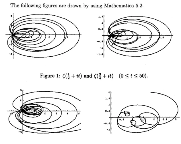
The following figures are drawn by using Mathematica 5.2.

Figure 1: $\zeta(\frac{1}{2}+it)$ and $\zeta(\frac{s}{4}+it)$ $(0\leq t\leq 50)$

.

Figure 2: $\zeta(\frac{1}{2}+it)$ and $\zeta(\frac{3}{4}+it)$ $(100000\leq t\leq 100010)$

.

Another conjecture closely related to (RH) is the so-called Lindel\"ofhypothesis

which is about how fast $\zeta(\sigma+it)$ grows

as

the imaginary part $t$ goes to $\infty$

.

We

define the order $\mu(\sigma)$

as

the least upper bound of the real numbers $c$ such that $|\zeta(\sigma+it)||t|^{-c}$ is bounded

as

$tarrow\infty$, i.e.,

$\mu(\sigma)=\lim_{tarrow}\sup_{\infty}\frac{\log|\zeta(\sigma+it)|}{\log t}$

For $\sigma>1$, it is obvious that $\mu(\sigma)=0$ because of (2). For $\sigma<0$, by the functional

equation (1) and the asymptotics of the F-function

$|\Gamma(s)|=(2\pi)^{1/2}(|t|+2)^{\sigma-1/2}e^{-\pi|t|/2}(1+O(|t|+2)^{-1}))$ uniformly for arbitrary strip $\sigma_{1}\leq\sigma\leq\sigma_{2}$, we get

$\zeta(\sigma+it)_{\wedge}\cdot(|t|+2)^{-\sigma+1/2}$ $(\sigma<0)$

.

Hence $\mu(\sigma)=-\sigma+1/2$ if$\sigma<0$. The remaining problem is to

see

what

occurs

in

between $0\leq\sigma\leq 1$

.

It is known that $\mu(\sigma)$ is non-negative, continuous and

(3)

order $\mu(\sigma)$ is

convex.

So

we can

conclude at least _{$\mu(\sigma)\leq(1-\sigma)/2$} if _{$0\leq\sigma\leq 1$}.

In particular, on the critical line $\sigma=1/2$, we have

$\zeta(1/2+it)\ll|t|^{1/4}$

.

Hardy-Littlewood showed that $\mu(\sigma)\leq 1/6=0.16666$, after that many

mathemati-cians improved again and again. So far, Huxley [4] has obtained the best result

$\mu(\sigma)\leq 32/205\fallingdotseq 0.156098$. The ultimate goal of this problem is considered

as

the

following.

(LH). The Lindel\"of hypothesis says that $\mu(1/2)=0$

.

In other words,

$\zeta(1/2+it)\ll|t|^{\epsilon}$ $\forall\epsilon>0$.

Remark. The Riemann hypothesis (RH) implies the Lindel\"of _{hypothesis (LH).}

In-deed, it is known that if(RH) is true, then

$\zeta(1/2+it)=O(\exp(c\frac{\log t}{\log\log t}))$

for

some

$c$, and it is stronger than (LH).

(LH) says thatthe Riemann-zeta function

grows

very slowly,

on

the other hand, it

is shown that for $1/2<\sigma\leq 1$, the set $\{\zeta(\sigma+it), t\in R\}$ is dense in $C$, and it is

believed that this is also the

case

for $\sigma=1/2$

.

2 Asymptotic

behavior of

the

variance

of

ran-domized values of Riemann’s

zeta function

The behavior of the mean-value, for example,

$\frac{1}{T}\int_{0}^{T}|\zeta(\sigma+it)|^{2k}dt$ $(k=1,2, \ldots)$

is easier to analyze than that of the order of $|\zeta(\sigma+it)|$ itself. The integral above

is considered

as

the $2k$-th moment of the random variable $\zeta(\sigma+iU)$ with uniform

random variable $U$

on

_{$[0, T]$}

,

and $\zeta(\sigma+it)$ is considered

as

a (trivial) stochastic

process $\{\zeta(\sigma+iS_{t}), t\geq 0\}$ with $\{S_{t}=t, t\geq 0\}$

.

It might be natural to study a

random varlable ($(\sigma+iX)$

or a

stochastic process $\{((\sigma+iS_{t}), t\geq 0\}$

.

Let $\xi_{1},$

$\ldots,$

$\xi_{n}$

are

i.i.$d$

.

Cauchy random variables whose probability law is given

by

$\frac{P(\xi_{1}\in dx)}{dx}=\frac{1}{\pi(1+x^{2})}$

and its characteristic function is $e^{-|\lambda|}$

.

The Cauchy random walk is defined

as

the

sum

of i.i.$d$

.

Cauchy random variables, _{$S_{n}=\xi_{1}+\cdots+\xi_{n},$} $n=1,2,$

(4)

and Weber [5] discussed the limiting behavior ofrandomized values of the Riemann zeta function

on

the critical line

$\zeta_{n}=\zeta(\frac{1}{2}+\dot{\iota}S_{n})$

sampled by the Cauchy random walk. The

mean

$E\zeta_{n}$ goes to 1

as

$narrow\infty$ (see (5)

below). For the second moment, they obtained the following results.

Theorem 1 ([5]). As $narrow\infty,$ $var(\zeta_{n})=$ log $n+A+o(1)$

.

The constant $A$ is

explicitly given

as an

integral.

Also, they show

an

almost

sure

convergence result for the

sum

of randomized

values.

Theorem 2 ([5]). For any real $b>2$,

$\sum_{k=1}^{n}\zeta(\frac{1}{2}+iS_{k})=n+o(n^{1/2}(\log n)^{b})$

as

$narrow\infty$

.

Since$\zeta(1/2+it)$ lives beyond the domain ofabsolutely

convergence,

we

cannot directly deal with the power series in the definition ofthe Riemann zeta function. The main idea of the proof ofthese results is to consider the random variable

$Z_{n}(x)= \sum_{k\leq x}k^{-\frac{1}{2}-iS_{n}}-\int_{0}^{x}u^{-\frac{1}{2}-iS_{\hslash}}du$

$= \sum_{k\leq x}k^{-}2\iota_{e^{i(-\log k)S_{n}}-}\int_{0}^{x}u^{-\frac{1}{2}}e^{i(-\log u)S_{n}}du$ (3)

which approximates$\zeta(1/2+iS_{n})$ by using the approximatefunctional equation due

to Hardy-Littlewood: Proposition 1. Let $x>1$

.

$\zeta(s)=\sum_{k\leq x}k^{-s}-\int_{0}^{x}u^{-\iota}ds+O(x^{-\sigma})$

uniformly

on

$\sigma_{0}\leq\sigma<1$ and $|t| \leq\frac{2\pi x}{c}$ with $C>1$

.

Proof.

See Theorem 4.11 in [10] and recall the identity

$\frac{x^{1-s}}{1-s}=\int_{0}^{x}u^{-s}ds$

(5)

When $S_{n}$ is the Cauchy random walk, all quantity such

as

the

mean

and the

variance for $Z_{n}(x)$

can

be computed explicitly (for example,

see

(5) below) and

that is

one reason

why they take up the Cauchy random walk.

We would like to

see

what happens if we replace the Cauchy random walk by

other stochastic processes. The natural candidate for this problem is the L\’evy

processes. In this note, we discuss the

same

problem

as

studied in [5] for a special

class of L\’evy processes, the symmetric $\alpha$-stable process with $1\leq\alpha\leq 2$ which

includes the Cauchy random walk

as a

special

case

of $\alpha=1$

.

Our

argument

goes

essentially parallel to [5] with

a

little

modification.

Here

we

recall the L\’evy

processes

(cf. [1, 9]). The L\’evy process $\{S_{t}, t\geq 0\}$ is

a

stochastic process which has stationary independent increments. The

outstand-ing feature coming from stationary independent increments is that there exists

a

function $\Psi(\lambda)$ such that the characteristic function is given by the formula

$Ee^{i\lambda S_{t}}=e^{-t\Psi(\lambda)}$ (4)

The function $\Psi(\lambda)$ is called the characteristicexponent and has theL\’evy-Khintchin

representation:

$\Psi(\lambda)=i\lambda a+\frac{c\lambda^{2}}{2}+\int_{R}(1-e^{i\lambda x}+i\lambda xI_{|x|\leq 1})\Pi(dx)$,

where $a\in R,$ $c\geq 0$ and $\Pi(dx)$ is the so-called L\’evy

measure

satisfying $\Pi(\{0\})=0$

and $\int_{R}$(1 A $x^{2}$)$\Pi(dx)<\infty$

.

The symmetric $\alpha$-stable process is the special

case

where

$\Psi(\lambda)=|\lambda|^{\alpha}$ $(0<\alpha\leq 2)$, $\Pi(dx)=|x|^{-\alpha-1}dx$ $(0<\alpha<2)$

.

The

case

$\alpha=1$ correspondstotheCauchy process and the

case

$\alpha=2$theBrownian

motion.

Remark. The symmetric$\alpha$-stable process is recurrent when $1\leq\alpha\leq 2$andtransient

when $0<\alpha<1$

.

By (3) and (4), it is

easy

to

see

that

$EZ_{t}(x)= \sum_{k\leq x}k^{-\frac{1}{2}}e^{-t\Psi(-\log k)}-\int_{0}^{x_{1}}u^{-\pi}e^{-t\Psi(-\log u)}du$

and, in particular, when $\alpha=1$, i.e., $\Psi(\lambda)=|\lambda|$, we

see

that

$\lim_{xarrow\infty}EZ_{t}(x)=\zeta(t+1/2)-\frac{2t}{t^{2}-1/4}$ (5)

$arrow 1$

as $tarrow\infty$

.

Remark that by the property that $\zeta(\overline{s})=\overline{\zeta(s)}$, the

mean

_{$E\zeta(\sigma+iX)$}

(6)

the

same

law. For a wide class of L\’evy processes

even

in the non-symmetric case,

$E\zeta(\sigma+iS_{t})$

goes

to 1

as

$tarrow\infty$

.

How well does the random variable $Z_{t}(x)$ approximate $\zeta(\frac{1}{2}+iS_{t})$?

Lemma 1. Suppose that $X$ is

a

random variable with density$p(x)$ which satisfies $p(x)$ $|x|^{-\gamma}$ with_$\gamma>1$

.

Then, _{$\zeta(1/2+iX)$}isan$L^{2}$ random variable. Furthermore,

there exists $M>0$ such that $p(x)$ is differentiable for $|x|>M$ and satisfies

$p(x)+ \int_{x}^{\infty}|p’(u)|du\ll|x|^{-\gamma}$ with$\gamma>3/2$, then $Z_{X}(x)$ converges to $\zeta(1/2+iX)$ in

$L^{2}$

as

_{$xarrow\infty$}, where _{$Z_{X}(x)$} is defined by (3) using _$X$ in place of _{$S_{n}$}

.

If

we

believe (LH), the integrability of$\zeta(1/2+iX)$ becomes much stronger. See Problem 3 below. We do not know whether (LH) is true,

so

instead, we use

a

mean

value theorem

$\int_{0}^{T}|\zeta(1/2+it)|^{2}dt\sim T$log$T$ $(Tarrow\infty)$

for the proof ofthis lemma.

FMrom

now

on,

we

consider the symmetric $\alpha$-process with $1\leq\alpha\leq 2$

.

Let $p_{t}(x)$

bethe transition density of the $\alpha$-stable process which is given by

$p_{t}(x)= \frac{1}{2\pi}\int_{R}e^{izx-t|z|^{\alpha}}dz=\frac{1}{\pi}\Re\int_{0}^{\infty}e^{izx-tz^{\alpha}}dz$

.

It is clear from the above that the transition density has the scaling property

$p_{t}(x)=t^{-1/\alpha}p_{1}(t^{-1/\alpha}x)$

.

As in [12], by using thecontour$\{z\in C;{\rm Im}(izx-z^{\alpha})=0\}$

,

Cauchy’s theoremgives

us

that

$p_{1}(x)= \frac{\alpha}{\pi(\alpha-1)}x^{\frac{1}{\alpha-1}}\int_{0}^{\pi/2}\varphi(\theta)$exp $(-x^{\underline{A}}\overline{\alpha}\overline{1}\varphi(\theta))d\theta$

and also

$p_{1}’(x)= \frac{-1}{\pi(\alpha-1)}x^{\frac{2}{\alpha-1}}\int_{0}^{\pi/2}r(\theta)^{2}(1-\frac{\alpha\sin(\alpha-2)\theta}{\sin\alpha\theta})\exp(-x^{\frac{\alpha}{\alpha-1}}\varphi(\theta))d\theta$

where

$r( \theta)=(\frac{\cos\theta}{\sin\alpha\theta})^{\frac{1}{\alpha-1}}$ , $\varphi(\theta)=r(\theta)^{\alpha}\frac{\cos(\alpha-1)\theta}{\cos\theta}$

.

The main contribution

comes

from

near

$\theta=\pi/2$

as

$xarrow\infty$,

we

see

that $p_{1}(x)+ \int_{x}^{\infty}|p_{1}’(u)|du\leq C|x|^{-\alpha-1}$

.

Hence, Lemma 1 shows that $Z_{t}(x)$ approximates$\zeta(1/2+iS_{t})$in $L^{2}$ andit is enough

(7)

$Remo,7^{\cdot}k$

.

For the case $0<\alpha<1$, there are similar integral representations for the

transition density by duality around $\alpha=1$.

Proposition 2. Let $S_{t}$ be the symmetric $\alpha$-stable process with $1\leq\alpha\leq 2$ and $\zeta_{n}=\zeta(1/2+iS_{n})$. Then, 下s $narrow\infty$

(i) $E\zeta_{n}=1+O(n^{-1/\alpha})$.

(ii) $var(\zeta_{n})=O(\log n)$

.

(iii) $cov(\zeta_{n}, \zeta_{m})=O(m^{-1/\alpha})\vee O(C_{\alpha}^{n-m})$ whenever $n>m$ for

some

$C_{\alpha}>0$

.

From this proposition, it is easy to

see

that

$var(\sum_{k=i}^{j}\zeta_{k})=\{\begin{array}{ll}O((j-i)j^{1-1/\alpha}) 1\leq\alpha\leq 2O((j-i)\log j) \alpha=1.\end{array}$

and

we

obtain the following almost

sure

convergence.

Theorem 3. Let $S_{t}$ be the symmetric $\alpha$-stable process with $1\leq\alpha\leq 2$

.

Then, $\sum_{k=1}^{n}\zeta(1/2+iS_{n})=n+o(n^{1-\Gamma^{1}\alpha}(\log n)^{b})$

for any $b>3/2$ if $1<\alpha\leq 2$; for any $b>2$ if $\alpha=1$

.

Although the random variables$\zeta_{n}-1,$$n=1,2,$ _$\ldots$ in

our

case are

not orthogonal

but weakly dependent,

an

extension of Rademacher-Menchoff type almost

sure

convergenoe theorem

can

be applied. Here

we

use a

simplified version ofa result

obtained in [11].

Proposition 3 ([11]). Let $\xi_{1},$$\xi_{2},$

$\ldots$ be randomvariables and $\Phi$ : $(0, \infty)arrow(0, \infty)$

a

concave

nondecreasing function. Suppose

$E| \sum_{1}^{j}\xi_{k}|^{2}\leq\Phi(j)(j-i)$

for any $1\leq i<j$

.

Then,

$\frac{\sum_{k--l}^{n}\xi_{k}}{(n\Phi(n))^{1/2}\log^{\tau}(1+n)}arrow 0$ _$a.s$

.

(8)

3 Some related

problems

Here we list

some

problems related to this topic.

Problem 1. What happens if we consider Dirichlet’s L-functions in plaoe of the

Riemann zeta function?

Problem 2. Lifshits and Weber gave the exact asymptotics of the variance in

Theorem 1, while here

we

just show $O(\log n)$ for it. Give theexact asymptoticsfor

the $\alpha$-stable

case.

Problem 3. Heuristically, (LH) implies that

$E|\zeta(1/2+iX)|^{p}\ll E|X|^{pc}<\infty$

if $\epsilon>0$ is arbitrary small. Does it hold that _{$\zeta(\frac{1}{2}+iX)\in\bigcap_{p>0}L^{p}$} for a random

variable $X \in\bigcup_{p>0}L^{p}$?

Problem 4. Here we only dealt with the

case

where $S_{t}$ is the $\alpha$-stable process

with $1\leq\alpha\leq 2$

.

As mentioned in the remark, the symmetric $\alpha$-stable process is

transient or recurrent according to $0<\alpha<1$

or

$1\leq\alpha<2$

.

Since the Lindel\"of

hypothesis corresponds tothedeterministic (transient) process$S_{t}=t$, the transient

case

should be more appropriate to study. What happens for the $\alpha$-stable process

with $0<\alpha<1$_{? Moreover, what} _happens _for $\alpha$-stable subordinator(increasing

L\’evy process) with $0<\alpha<1$ or, furthermore, for general L\’evy processes?

Problem 5. Related to Problem 4, we consider the Brownian motion $S_{t}$ with

constant drift whose characteristic exponent is $\Psi(\lambda)=\epsilon\lambda^{2}/2+ia\lambda(\epsilon>0, a\in R)$

.

In thiscase,

we

can

compute directly themoments of$\zeta(1/2+iS_{t})$ by using another

integral representation of the Riemann zeta function

$\zeta(s)=s\int_{0}^{\infty}Q(x)x^{-(s+1)}dx$ $(0<\Re s<1)$

where $Q(x)=[x]-x$

.

If$E|S_{t}|<\infty$,

$E \zeta(\sigma+iS_{t})=\int_{-\infty}^{\infty}Q(e^{-u})e^{\sigma u}(\sigma-t\Psi’(u))e^{-t\Psi(u)}du$

and if $S_{t}$ is the Brownian motion with constant drift

$E[|\zeta(\sigma+iX_{t})|^{2}]$

(9)

In particular, when $\Psi(\lambda)=\frac{\epsilon\lambda^{2}}{2}+ia\lambda$, setting $b=\epsilon^{-1}a$ and $T=t\epsilon$,

we

obtain $E[| \zeta(\sigma+iX_{t})|^{2}]=2\int_{0}^{\infty}Q(x)x^{-(1+2\sigma)}dx\cross\int_{0}^{\infty}Q(xe^{-u})e^{\sigma u}f(u;T, b)e^{-\tau_{\tau^{-du}}^{u^{2}}}$

where

$f(u;T, b)=(\sigma^{2}+T-T^{2}(u^{2}-b^{2}))\cos(h\iota T)-2T^{2}ubs\ln(buT)$

.

Compute the

as

ymptotic behavior of the second moment

as

$Tarrow\infty$, especially

when $b$ is

non-zero.

Problem 6. It is well-known that (LH) is equivalent to

one

of the following

con-ditions 1. $E[|\zeta(1/2+iU_{T})|^{2k}]=O(T^{\epsilon})$, $k=1,2,$ _$\ldots$ 2. $E[|\zeta(\sigma+iU_{T})|^{2k}]=O(T^{\epsilon})$, $\sigma>\frac{1}{2},$$k=1,2,$ $\ldots$ 3. $\lim_{arrow\infty}E[|\zeta(\sigma+iU_{T})|^{2k}]=\sum_{n=1}^{\infty}\frac{d_{k}^{2}(n)}{n^{2\sigma}}$ , $\sigma>\frac{1}{2},$$k=1,2,$ $\ldots$

where $U_{T}$ is

a

random variable uniformly distributed

on

$[0,T]$ and _{$d_{k}(n)$} denotes

the number ofways of representing integer $n$ \"as aproduct of$k$ factors. What kind

of family ofrandom variables has the

same

property

as

$\{U_{T}, T\gg 1\}$ does.

Problem 7. It is known that $\frac{\log\zeta(l/2+1U_{T})}{\sqrt{}\log\log T}arrow N_{C}(0,1)$

as

$Tarrow\infty$ where $U_{T}$ is

dis-tributeduniformly

on

$[0,T]$ (cf. [3]). Discusslimittheorems

or

the largedeviations

for the process $\{\zeta(1/2+iS_{t}), t\geq 0\}$

or

$\{\log\zeta(1/2+iS_{t}), t\geq 0\}$

.

Problem 8. The following normalized zeta function

$\xi(s)=\frac{1}{2}s(s-1)\pi^{-s/2}\Gamma(\frac{s}{2})\zeta(s)$

.

is sometimes used. This is

an

entire

function

which

satisfies

the following simple functional equation:

$\xi(s)=\xi(1-8)$

.

One of the important feature of this version is that it is real-valued

on

the critical lIne. This function is related to probabilIty theory in this way: let $Y$ be

a

random variable defined by

$Y=\sqrt{\frac{2}{\pi}}(\max_{0\leq*\leq 1}b_{\epsilon}-\min_{0\leq s\leq 1}b_{l})$

where $\{b_{s}, 0\leq s\leq 1\}$ is the standard Brownian bridge pinned at $(t, x)=(0,0)$

(10)

connection between this random variable and the Riemann zeta function is given

by the following relation

$EY^{s}=2\xi(s)$ $(s\in C)$ Another related random variable is

defined

by

$S= \frac{2}{\pi^{2}}\sum_{n=1}^{\infty}\frac{\gamma_{n}}{n^{2}}$

where $\{\gamma_{n}, n=1,2, \ldots\}$

are

i.i.$d$

.

random variables such that the density $P(\gamma_{1}\in$

$dx)/dx=xe^{-x}$

.

It is known that

$Y=d(\frac{\pi}{2}S)^{1/2}$

.

See [2] for this topic. Are there any approaches to the growth problem by using

this probabilistic interpretation?

References

[1] J. Bertoin, L\’evy Processes, Cambridge tracts in mathematics 121, Cambridge University Press, 1996.

[2] P. Biane, J. Pitman and M. Yor, Probability laws related to the Jacobi theta

and Riemann zeta functions, and Brownian excursions, Bull. Amer. Math.

Soc. 38 (2001), 435-465.

[3] C. P. Hughes, A. Nikeghbali and M. Yor, An arithmetic model for the total

disorder process, available via $arXiv:math.PR/0612195vl$

.

[4] M. N. Huxley, Exponential

sums

and the Riemann zeta function V, Proc.

London Math.

Soc.

90 (2006), 1-41.

[5] M. Lifshits and M. Weber, Sampling the Lindel\"ofhypothesis with the Cauchy random walk, available via $arXiv:math.PR/0703693vl.$.

[6] K. Matsumoto, The Riemann Zeta Function (in Japanese), Asakura-Syoten,

2005.

[7] K. Sato, L\’evy Processes and Infinitely Divisible Distributions, Cambridge

studies in advanced mathematics 68, Cambridge University Press,

1999.

[8] T. Shirai,

On

the randomized values of Riemann’s zeta function

on

thecritical

line, in preparation.

[9] W. F. Stout, Almost Sure Convergence, Probability and Mathematical$Stati*$

(11)

[10] E. C. Titchmarsh, The theory of the Riemann Zeta-function, Oxford, 1951.

(2nd ed., revised by D.R.Heath-Brown, Oxford, 1986. )

[11] M. Weber, Uniform bounds under increment conditions, functions, Trans.

Amer. Math. Soc.

358

(2006),

911-936.

[12] V. M. Zolotarev, One-Dimensional Stable Distributions, Amer. Math. Soc., Providence, RI.,