Analytical derivation of diffusion coefficient of two-dimensional point vortex system with Klimontovich formalism (Modern approach and developments to Onsager's theory on statistical vortices)

Analytical derivation of diffusion coefficient

of

two-dimensional

point

vortex

system with

Klimontovich

formalism

Yuichi

YATSUYANAGI

Faculty

of

Education,

Shizuoka

University

Tadatsugu

HATORI

Faculty of

Science, Kanagawa University

1

Introduction

A diffusion coefficient of a two-dimensional (2D) point vortex system is analytically

derived with Klimontovich formalism.

The main motif of this international seminar is to provide

an

opportunity for

collab-oration between mathematician and physicist. In such case, jargons in

a

group prevent

the other group from active discussion. So, I will try to explain meanings of the words

which may be potentially jargons.

The $2D$ inviscid Euler equation has

a

formal solution ofsingular point _vortices.

How-ever, the Euler equation is the macroscopic fluid equation and should have macroscopic

smooth solutions. We regard the Euler equation that has the singular point vortex

solu-tion

as a

kineticequation. Thekinetic equationis formally identicalwith themacroscopic

Eulerequation. It happens that the macroscopic Euler equation and thekinetic equation

have the

same

form.

Similar

case

can

be found in plasmaphysics. The Klomontovich-Dupree equation is

a

kineticequationthat has a discretized exactsolutionbythe Diracdeltafunctionin

a

phase

space. Bycoarse-graining (averaging) the equation, the Fokker-Plancktypecollisionterm

is obtained. A kinetic equation with the Fokker-Planck type collision term is called the

Fokker-Planck equation, which is the versionofthe Boltzmann equation applicable to the

case

of long-range interparticle forces. The above procedure is called the Klimontovich

formalism. This time,

we

apply the Klimontovich formalism to the point-vortex system,

The organization

of

this paper is

as

follows: In

Sec.

2, the point vortex system is

introduced. In

Sec.

3, outlineof the Klimontovich formalismis given. In

Sec.

4

our

result

will be given. In Sec. 5 we give

our

conclusion.

2

Point

vortex

system

The$2D$ Eulerequationis

a

partial

differential

equationwhich describes incompressible

flow in $2D$ plane.

$\frac{\partial u(r,t)}{\partial t}+u(r, t)\cdot\nabla u(r, t)=0$. (1)

Thevorticity equation is obtained by taking the rotation differential:

$\frac{\partial\omega_{z}(r,t)}{\partial t}+u(r, t)\cdot\nabla\omega_{z}(r, t)=0$, (2)

and it has a point vortex solution:

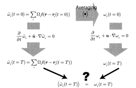
$\omega_{z}(r, t)=\sum_{i}\Omega_{i}\delta(r-r_{i}(t))$, (3)

where$\omega_{z}(r, t),$ $u(r, t)$

are

the

nonzero

component of the vorticity and the flow field in $2D$

plane pointedby$r=(x, y)$

.

The

circulation

(strength) of the i-th point vortex at position

$r_{i}$ is denotedby$\Omega_{i}$ whose valueiseither $\Omega_{0}or-\Omega_{0}$ where $\Omega_{0}$ is

a

positiveconstant. This

solution (3) is discretized by the Dirac delta function. In general, macroscopic fluid

equation should have

a

smooth solution. Thus,

we

regard the point vortex solution is

a

solution for

a

kinetic equation that is formally identical with the $2D$ Euler equation. We

call this equation the microscopic Euler equation. To distinguish the microscopic Euler

equation from the macroscopic one,

we

indicate the microscopic variable with a hat.

$\frac{\partial\hat{\omega}_{z}(r,t)}{\partial t}+\hat{u}(r, t)\cdot\nabla\hat{\omega}_{z}(r, t)=0$ (4)

Themicroscopic and macroscopic variables

are

related by (ensemble)

average

operator $\{\cdot\rangle$

$\omega_{z}(r, t)=\{\hat{\omega}_{z}(r, t)\}$. (5)

The microscopic vorticity $\hat{\omega}_{z}(r, t)$, velocity$\hat{u}(r, t)$ and stream function$\hat{\psi}(r, t)$ satisfy the

following relations,

$\hat{u}(r, t)$ $=$ $\nabla\cross(\hat{\psi}(r, t)\hat{z})=-\hat{z}\cross\nabla\hat{\psi}(r, t)$ , (6)

$\hat{\omega}_{z}(r, t)$ $=$ $\nabla\cross\hat{u}(r, t)=-\nabla^{2}\hat{\psi}(r, t)$ (7)

where $\hat{z}$ is

a

unit vector in

$z$ direction. Positions of the point vortices

are

governed

by the microscopic Euler equation and by coarse-graining the distribution ofthe point

vortices, macroscopic vorticity distribution $\omega_{z}(r, t)$ is obtained. Here,

a

question arises.

Themicroscopicsolutiongoverned bythemicroscopic Eulerequationandthe macroscopic

solution governed by the macroscopic Euler equation is the

same

as

is shown in Fig. 1?

$l$

$\{\hat{\omega}_{z}(t=T)\}$ $=$ $\omega_{z}(t=T)$

Figure 1: The microscopic solution governed by the microscopic Euler equation and the

macroscopic solution governed by the macroscopic Euler equation is the same?

3

Klimontovich formalism

Klimontovich-Dupree equation

$\frac{\partial\hat{f}(r,v,t)}{\partial t}+v\cdot\nabla\hat{f}(r, v, t)+\frac{q}{m}(\hat{E}+v\cross\hat{B})\cdot\frac{\partial}{\partial v}\hat{f}(r, v, t)=0$ (8)

is

an

equation for 6-dimensional phase space with $(r, v)$ and has

an

exact solution for

a

particle density function $\hat{f}(r, v, t)[1]$.

$f(r, v, t)= \sum_{i}\delta(r-r_{i}(t))\delta(v-v_{i}(t))$ (9)

The hat on the particle density function $f$

means

this function microscopic. The

mi-croscopic electric and magnetic fields $\hat{E}$ and $\hat{B}$ obey the microscopic Maxwell equation

that is identical withthe macroscopic (usual) Maxwell equation

as

the Maxwell equation

does not have nonlinear term. It is assumed that the microscopic quantity consists of a

macroscopic part and a fluctuation.

$f(r, v, t)$ $=$ $\{f(r, v, t)\}+\delta f(r, v, t)=f(r, v, t)+\delta f(r, v, t)$ (10)

$\hat{E}(r, v, t)$ $=$ $E(r, v, t)\}+\delta\hat{E}(r, v, t)$ (11)

$\hat{B}(r, v, t)$ $=$ $B(r, v, t)+\delta\hat{B}(r, v, t)$ (12)

Note that a macroscopic quantity is obtained by averaging

a

microscopic quantity with

Figure 2: Klimontovich equation is related to the microscopic Euler equation that has the point vortex solution. By averaging Klimontovich equation, macroscopic

Fokker-Planck equation is obtained. Ignoring the Fokker-Planck collision term,

Vlasov

equation

isobtained.

We

regard that the macroscopic Euler equationis related to themacroscopic

Vlasov equation. There is

no

related equation for the Fokker-Planck equation.

(13)

Klimontovich-Dupree equation and averaging the equation, the following macroscopic

equation is

obtained.

$\frac{\partial f}{\partial t}+v\cdot\nabla f+\frac{q}{m}(E+v\cross B)\cdot\frac{\partial f}{\partial v}=\frac{q}{m}\{(\delta\hat{E}+v\cross\delta\hat{B}\cdot\frac{\partial}{\partial\delta v}\delta\hat{f})\}$

Further calculation yields the Fokker-Planck collision term from the right hand side of

Eq. (13) and

a

kinetic equation with Fokker-Planck collision term is called

Fokker-Planck

equation:

$\frac{\partial f}{\partial t}+v\cdot\nabla f+\frac{q}{m}(E+v\cross B)\cdot\frac{\partial f}{\partial v}=\frac{\partial}{\partial v}\cdot(\overline{D}\cdot\frac{\partial f}{\partial v})$. (14)

If the collision term is dropped completely, it iscalled Vlasov equation:

$\frac{\partial f}{\partial t}+v\cdot\nabla f+\frac{q}{m}(E+v\cross B)\cdot\frac{\partial f}{\partial v}=0$ (15)

We summarize the relation between the Klimontovich equation and the point vortex

equation in Fig. 2. Klimontovich equation is related to the microscopic Euler equation

that has the point vortex solution. By averaging Klimontovich equation, macroscopic

Fokker-Planck equation is obtained. Ignoring the Fokker-Planck collision term, Vlasov

equation is obtained. We regard that the macroscopic Euler equation is related to the

macroscopicVlasovequation. There is

no

relatedequationfor the Fokker-Planckequation.

This time,

we

focus ourselvesto obtainthe corresponding macroscopic equation that may

4

Kinetic

theory

for

$2D$

point

vortex

system

To obtain the Fokker-Planck type collision term for the $2D$ point vortex system, the

same

procedure

as

the Klimontovich formalism is applied. Microscopic vorticity is

as-sumed to consist of the macroscopic vorticity and the fluctuation.

$\hat{\omega}_{z}(r, t)$ $=$ $\{\hat{\omega}_{z}(r, t)\}+\delta\hat{\omega}_{z}(r, t)=\omega_{z}(r, t)+\delta\hat{\omega}_{z}(r, t)$ (16)

$\hat{u}(r, t)$ $=$ $u(r, t)+\delta\hat{u}(r, t)$ (17)

Same

as

before, substituting the microscopic variables into the microscopic Euler equation and averaging it, the following macroscopic equation is obtained.

$\frac{\partial\omega_{z}(r,t)}{\partial t}+u(r, t)\cdot\nabla\omega_{z}(r, t)=-\nabla\cdot\langle\delta\hat{u}(r, t)\delta\omega_{z}(r, t)\rangle$ (18)

To evaluate the diffusion term

on

the right hand side,

we

need

an

evolution equation

for $\delta\omega_{z}(r, t)$

.

For this purpose, linearlized equation is introduced, which is obtained by

substituting the microscopic variables (16) and (17) into the microscopic Euler equation

(4) and dropping the zero-th ordermacroscopic terms. The obtained linearlized equation

is given by

$\frac{\partial}{\partial t}\delta\hat{\omega}_{z}(r, t)+u(r, t)\cdot\nabla\delta\hat{\omega}_{z}(r, t)=-\delta\hat{u}(r, t)\cdot\nabla\omega_{z}(r, t)$ . (19)

This linearlized equation can be integrated as$u(r, t)$ _{in the second term} on the left hand

side and $\omega_{z}(r, t)$

are

assumed to be constant in the microscopic scale:

$\delta\hat{\omega}_{z}(r, t)=-\int_{-\infty}^{t}d\tau\delta\hat{u}(r-(t-\tau)u, \tau)\cdot\nabla\omega_{z}(r, t)$ (20)

Finally, the corresponding macroscopic equation is obtained:

$\frac{\partial}{\partial t}\omega_{z}(r, t)+u(r, t)\cdot\nabla\omega_{z}(r, t)=\nabla\cdot(\etarightarrow\cdot\nabla\omega_{z}(r, t))$ (21)

$\etarightarrow=\int_{-\infty}^{t}\langle\delta\hat{u}(r, t)\delta\hat{u}(r-(t-\tau)u, \tau)\}d\tau^{\sim}$ (22)

The right hand side is the diffusion term due to the discreteness of the vorticity. It may

be

an

extension of the well-known Green-Kubo formula. This result includes the position

and time correlations, while

Green-Kubo formula

includes the time correlation only.

5

Conclusion

We have derived the diffusion term implicitly included in $2D$ Euler equation. On the

In

general,

collision

term in

Fokker-Planck

equation consists

of

two parts:

the diffusion

term and the friction term.

$\nabla\cdot(\etarightarrow\cdot\nabla\omega_{z}+A\omega_{z})$ (23)

In

our

result, friction term is not included. The frictiontermmay be derived by rewriting

Eq. (20)

as

$\delta\hat{\omega}_{z}(r, t)$ $=$ $- \int_{t_{0}}^{t}d\tau\delta\hat{u}(r-(t-\tau)u, \tau)\cdot\nabla\omega_{z}(r, t)$

$+\delta\omega_{z}(r-(t-t_{0})u, t_{0})$. (24)

Further calculation reveals that the second term is proportional to $\omega_{z}$. As this effect is,

however, evaluated negligible

as

compared with the diffusion term,

we

ignore the term.

References

[1] Y. L. Klimontovich: The

statistical

theory

_of

non-equilibrium processes in

a

plasma