On the influence of delay to the strength of oscillation criteria for neutral second order half-linear differential equations (Qualitative theory of ordinary differential equations in real domains and its applications)

(1)

On

the influence of delay

to

the strength of oscillation

criteria

for

neutral second

order

half-linear diﬀerential

equations

Robert

Ma\v{r}\’ik

Department

of

Mathematics, Mendel

University

in

Brno

Abstract

In the paperwestudythe second order neutral delay half-linear diﬀerential equation

$[r(t)\Phi(z’(t))]’+q(t)\Phi(x(\sigma(t)))=0,$

where$\Phi(t)=|t|^{p-2}t,$$p\geq 2$and$z.(t)=x(t)+b(t)x(\tau(t))$. We summarizethreediﬀerent methods availableto derive oscillationcriteriafor thisequationand comparethemonthe particular

ex-ampleof Eulertype equation and proportional delay. We show thatfor thisparticular equation the comparisonmethodproducesbetterresults ifthe delay is significant, whereasRiccati

equa-tionmethod produces sharper results if the delay argument is close to the classical argument.

We alsopoint outsome recentdevelopment in this area.

Keywords: half-linear diﬀerential equation, oscillation criteria, Riccati technique, delay

equa-tion, neutral equaequa-tion, Euler type equation

MSC: $34K11,$ $34K40$

1 Introduction

Consider the second order half-linearneutral diﬀerentialequation

$[r(t)\Phi(z’(t))]’+c(t)\Phi(x(\sigma(t)))=0, z(t)=x(t)+b(t)x(\tau(t))$, (1)

where $\Phi(t)=|t|^{p-2}t$ _{is the power type nonlinearity}_and$p\geq 2$,whichensures thatthefunction$\Phi$

is aconvex functionon $(0, \infty)$.

Underthe solutionof (1) we understand anydiﬀerentiable function$x(t)$ _{which does}_not

identi-cally equal zero $eventually_{\rangle}$ such that$r(t)\Phi(z’(t))$ _is _{diﬀerentiable}_{and (1)} _holds _{for large} $t.$

The solution ofequation (1) is said to be oscillatory ifit has infinitely many zeros tending to

infinity. Equation (1) issaidto beoscillatory ifallitssolutions areoscillatory. Inthe opposite$case_{\}}$

i.e., if there exists aneventually positive solution of (1), equation (1) is said to be nonoscillatory.

There

are

many oscillation criteria forequation (1) obtained byanapplicationofessentiallyone

(2)

(i) using comparison with

a

half-linear second order equation based

on

apriori bound for the

quotient $x(t)/z(t)$ (see e.g. [2,8,18

(ii) using the comparison method (comparison with linear first order delay diﬀerential equation,

see

e.g. [4-7, 9, 11, 13, 15]) and

(iii) using the Riccati type substitution (seee.g. [10,14,17

The underlyingprincipleof all methods is toreplacetheequation (1) by

a

simpler object. The

specialfocus is usually devoted to the second term, since the most disturbing thing in equation (1)

isthe presenceof both $z(t)$ and$x(t)$ in oneequation_and _{it is easier} _to _eliminate$x$ than$z.$

It is typical that all new criteria published in the literature

are

compared against the criteria

obtained by the

same

method. The aim of this paper is to collect available methods whichcan be

used to derive oscillation criteria for equation (1) and compare them together. On

a

test of Euler

type equation wewill show that one ofthe methods produces sharper results for small delays and

another

one

for large delays. We will also modify the currently used approach in (i) and derive a

result whichis based on the comparison with second order delay diﬀerential equation rather than

second order ordinary diﬀerentialequation.

We will use the following assumptions on the coeﬃcients and parameters. The coeﬃcients $r$

and $b$

are

subject of usual conditions $r\in C^{1}([t_{0}, \infty), \mathbb{R}^{+})$, $b\in C^{1}([t_{0}, \infty), \mathbb{R}_{0}^{+})$ and the coeﬃcient

$c$ ispositive $c\in C([t_{0}, \infty), \mathbb{R}^{+})$

.

Further wesuppose that the deviating argumentsare unbounded,

increasing and suﬃciently smooth functions whichsatisfythe commutative law: $\tau\in C^{2}([t_{0}, \infty), \mathbb{R})$, $\tau’(t)>0,$ $\lim_{tarrow\infty}\tau(t)=\infty,$ $\sigma\in C^{1}([t_{0}, \infty), \mathbb{R})$, $\sigma’(t)>0,$ $\lim_{tarrow\infty}\sigma(t)=\infty$ and $\sigma(\tau(t))=\tau(\sigma(t))$

(for the weaker assumption $\sigma(\tau(t))\geq\tau(\sigma(t))$ see [10]). Depending on the method which will be

used to handle the problem, we will use some additional conditions,such

as

$b(t)\leq b_{0}$ or _$b(t)<1.$

For simplicity we will also suppose that both $\sigma$ and $\tau$ are delays and that the retardation in the

diﬀerential term is smaller than the retardation in the second term, i.e. we will suppose $\sigma(t)\leq$

$\tau(t)\leq t.$

In the paper the number $q=\overline{p}\overline{1}\underline{\not\simeq}$ is the conjugate numberto the number $p$. Given a positive

parameter $\varphi$ further define the function $Q$

as

minimum of$c(t)$ and$\varphi c(\tau(t))$

$Q(t; \varphi)=\min\{c.(t), \varphi c(\tau(t))\}$ (2)

Finally, we willuse the assumption

$\int^{\infty}r^{1-q}(t)dt=\infty$ ₍₃₎

which (together with nonnegativity of $c(t)$)

ensures

that all eventually positive solutions satisfy

$z’(t)>0$ eventually,

see

Lemma 1 below. Thus there is only one family of solutions which has

to be eliminated in order to

ensure

oscillation. Note that the opposite

case

to (3) is also handled

frequently in the literature and since in that case wehaveto eliminate two typesofsolutions(with

$z’(t)>0$ and $z’(t)<0$ eventually), the resulting oscillation criteria consist of two (similar but

relativelyindependent) conditions–each condition eliminates one of the families.

2 Monotonocity lemma

Thefollowinglemma

ensures

that theeventually positivesolutionssatisfy $z’(t)>0$ for large$t$. The

proofutilizes the condition (3) and can be found in many papers dealing with oscillation criteria

(3)

Lemma 1.

_If

$x(t)$ _is an eventually nonoscillatorysolution

of

(1), then the corresponding

function

$z(t)=x(t)+b(t)x(\tau(t))$

_satisfies

$z(t)>0, z’(t)>0, (r(t)\Phi(z’(t)))’<0$

eventually.

3 Method of apriori bound

The first idea how to remove the simultaneous presence of both $x(t)$ and $z(t)$ _{in (1) is} to replace

$x(\sigma(t))$ by alower bound interm of$z(\sigma(t))$

.

If $x(t)$ is eventually nonegative, _then $x(\tau(t))$ is also eventually nonegative and since $z(t)$ is

increasing and clearly $z(t)\geq x(t)$, wehave

$z(t)=x(t)+b(t)x(\tau(t))\leq x(t)+b(t)z(\tau(t))\leq x(t)+b(t)z(t)$

.

Thus if$b(t)<1$,the resulting inequalitycanbe utilizedtoobtainthe apriori boundfor thequotient

$x(t)/z(t)$

$0<1-b(t) \leq\frac{x(t)}{z(t)}$

.

(4)

Thisapproachis summarized in the following lemma. The special case$\eta(t)=a(t)$ hasbeenused in

most papers dealingwith themethod ofapriori bound. The idea toreplace $\sigma$by asmallerfunction

$\eta$(andthusincreasethe delay$t-\sigma(t)$)isnewbut verysimpleand allows toimproveresultsobtained

by an applicationofathe so-called Myshkis-typecriterion from Theorem 1 below.

Lemma 2. Let $\eta(t)$ be continuous

function

such that$\eta(t)\leq\sigma(t)$ and $\lim_{tarrow\infty}\eta(t)=\infty$

.

Suppose

that

$b(t)<1$ (5)

holds eventually and suppose that the inequality

$[r(t)\Phi(z’(t))]’+c(t)(1-b(\sigma(t)))^{p-1}\Phi(z(\eta(t)))\leq 0$ ₍₆₎

doesnot have an eventually positive solution. Then (1) is oscillatory.

Proof.

It is suﬃcient to show that if$x(t)$ is an eventually positive solution of (1), then the

corre-spondingfunction $z(t)$ satisfies (6) eventually. If$\eta\equiv\sigma$, then (6) follows immediately from (1) and

inequality (4). Thefact that $\sigma(t)$ can be replaced by $\eta(t)\leq\sigma(t)$ follows from the monotonicityof

the function $z(t)$, see Lemma 1. $\square$

Inequality (6) is the second order delay diﬀerential inequalitywhich does not contain delay in

the diﬀerential term and is not neutral anymore. If$p=2$, then this inequality is handled by the

following theorem ofKoplatadze.

Theorem 1 ([12, Theorem 2]). Let

(4)

Then the inequality

$x”(t)$_sgn$x(\eta(t))+c(t)|x(\eta(t))|\leq 0$

is oscillatory.

Note thatthe constant $\frac{1}{e}$ isoptimal and cannot be improved in general, but in

some

particular

cases a refinement of Koplatadze’s results is possible,

see

[16]. As a consequence of Theorem 1, equation

$x”(t)+ \frac{\beta}{t^{2}}x(\lambda t)=0$

is oscillatory if

$\beta>\frac{l}{e\lambda\ln\frac{1}{\lambda}}$ (7)

holds. You may

see

that the right hand side of thisinequality becomes unbounded if$\lambda$ approaches

1. This undesired eﬀectcan be eliminated by suitable choice of the function $\eta$ from Lemma 2,

see

(24) below.

Theorem 1 cannot be applied in the general

case

$p\geq 2$. Inthis

case

it is possibleto

use

another

apriory bound

$k \frac{\sigma(t)}{t}\leq\frac{z(\sigma(t))}{z(t)}$ for arbitrary $k\in(0,1)$ and large $t$ (8)

or

$\frac{\sigma(t)}{t}\leq\frac{z(\sigma(t))}{z(t)}$ for large$t$ (9)

which holds if

$\int^{\infty}c(s)(1-b(\sigma(s)))^{\rho-1}(\sigma(s))^{p-1}ds=\infty$, ₍₁₀₎

see [8, Theorem 13] for details.

Thus(6) does not haveaneventuallypositivesolutionifthecorresponding equationisoscillatory

which is true if either

$[r(t) \Phi(z’(t))]’+kc(t)(1-b(\sigma(t)))^{p-1}(\frac{\sigma(t)}{t})^{p-1}\Phi(z(t))=0$ ₍₁₁₎

is oscillatory for

some

$k\in(O, 1)$, or if (10) holds and

$[r(t) \Phi(z’(t))]’+c(t)(1-b(\sigma(t)))^{p-1}(\frac{\sigma(t)}{t})^{p-1}\Phi(z(t))=0$ ₍₁₂₎

is oscillatory.

Various oscillation criteria for half-linear ordinary diﬀerential equations (12) and (11) are in

details discussedin the book [3] which

covers

main directions in oscillation theory of thehalf-linear

(5)

4 Comparison

method

Themain idea of the comparisonmethod is to compare equation (1) with certainfirst order delay

diﬀerential inequality. Consider the original equation (1) and the same equation shifted from $t$

to $\tau(t)$

.

This gives in the second term expressions involving_{$x(\sigma(t))$}

and $x(\sigma(\tau(t)))$ which can be

combined into $z(\sigma(t))$. This allows to eliminate $x(t)$ _{in equation (1)} _{and introduce} $z(t)$ instead.

More precisely, weconsider theequation (1) and the equation

$\frac{1}{\tau’(t)}[r(\tau(t))\Phi(z’(\tau(t)))]’+c(\tau(t))\Phi(x(\sigma(\tau(t))))=0$ ₍₁₃₎

which arisesfrom (1) byshifting from $t$ to $\tau(t)$

.

Thenwetakeasuitablelinear combination of both

equations and use aseries of estimates which allow tocompare the resultingequation with certain

first order linear diﬀerential inequality. Note that the mainsteps to accomplish the desired result

are

inequality

$c(t)x^{p-1}( \sigma(t))+c(\tau(t))b_{0}^{p-1}x^{p-1}(\sigma(\tau(t)))\geq\min\{c(t)$,$c(\tau(t))\}(x^{p-1}(\sigma(t))+b_{0}^{p-1}x^{p-1}(\sigma(\tau(t))))$

(14)

followed by the assumptionon commutativitybetween $\tau$ and $\sigma$ and by inequality

$x^{p-1}(\sigma(t))+b_{0}^{p-1}x^{p-1}(\tau(\sigma(t)))\geq 2^{p-2}(x(\sigma(t))+b_{0}x(\tau(\sigma(t)))^{p-1}\geq 2^{p-2}z^{p-1}(\sigma(t))$_, ₍₁₅₎

where $b_{0}$ is aconstant upper bound of the function _$b(t)$.

A closer examination of the published results shows, that theseinequalities

are

in some sense

weakpointsofthe comparison method andpossessomeimprovement. See[10] for detailed discussion

and also for

more

generalversion of theseinequalities andsee also [8] forapplication of these ideas

to the equation(1) and thecomparison method. One of the main results of [8] states thefollowing.

Theorem 2 $($ [8, Corollary (9), statement (ii)]$)$

.

Suppose that there exists a number$b_{0}$ such that

$b(t)\leq b0$

.

Equation (1) is _oscillatory

_if

_there _exists _{a number}_$\varphi>0$ _and _a

function

$\eta(t)$ satisfying

$\eta(t)\leq\sigma(t)$ and$\lim_{tarrow\infty}\eta(t)=\infty$ such that_{$\eta(t)<\tau(t)\leq t$} _and

for

every$T$ there _exists $t_{1}$ such that

$\lim inftarrow\infty\int_{\tau^{-1}(\eta(t))}^{t}Q_{\eta}^{*}(s;\varphi, t_{1})ds>\frac{1}{e}(1+(\frac{\varphi}{\tau_{0}})^{q-1}b_{0})^{p-1}$ ₍₁₆₎

where

$Q_{\eta}^{*}(t; \varphi, t_{1}):=Q(t;\varphi)[\int_{t_{1}}^{\eta(t)}r^{1-q}(s)ds]^{p-1}$

Observe the presence of the function $\eta(t)$ in Theorem 2. An absolute _majority _of _{the recent}

papers does not consider function like $\eta$ in the comparison method and deal just with the special

case $\eta(t)=\sigma(t)$. However, the influence _of$\eta(t)$ to the value of the limes inferior on the left hand

side of the inequality (16) is ambivalent: bigger$\eta$ givesbigger$Q^{*}$ and thus has apositive influence

on the condition (16), but bigger $\eta$ also makes the interval of integration in (16) shorter and this

has anegative influence on the condition (16). As a consequence, some of the oscillation criteria

obtained by comparison method which produce poor results if $\sigma(t)$ is close to $t$ or $\tau(t)$ can be

improved byasuitable choiceof$\eta(t)<\sigma(t)$, seethe examples withsome discussion _{in [10,} _Example

2 andFigure 1], [9, Example 10 andFigure 2]. Asfar as the authorknows, theonlypapers dealing

(6)

5 Riccati equation method

The Riccati equation method is basedon the Riccati type substitution

$\omega(t)=\rho(t)\frac{r(t)(z’(t))^{p-1}}{z^{p-1}(\sigma(t))}$

.

(17)

which implies

$\omega’(t)=\rho’(t)\frac{r(t)(z’(t))^{p-1}}{z^{p-1}(\sigma(t))}+\rho(t)\frac{(r(t)(z’(t))^{p-1})’}{z^{p-1}(\sigma(t))}-(p-1)\rho(t)\frac{r(t)(z’(t)(\sigma(t))\sigma’(t)}{))}.$

From$\sigma(t)\leq t$ and from the monotonicity of$r(t)\Phi(z’(t))$ wehave

$z’( \sigma(t))\geq(\frac{r(t)}{r(\sigma(t))})^{q-1}z’(t)$

andcombining these computations with (1)

we

get

$\omega’(t)-\frac{\rho’(t)}{\rho(t)}\omega(t)+\frac{(p-1)\sigma’(t)}{\rho^{q-1}(t)r^{q-1}(\sigma(t))}\omega^{q}(t)\leq-\rho(t)\frac{c(t)x^{p-1}(\sigma(t))}{z^{p-1}(\sigma(t))}$. (18)

Notethat to perform these steps it is necessary tosuppose diﬀerentiability of$\sigma(t)$ and$\sigma(t)\leq t.$

Togetherwiththiscomputation

we

derive

a

variantofthelastinequality whichcontains$x^{p-1}(\tau(\sigma(t)))$

instead of$x^{p-1}(\sigma(t))$

.

Thenwewill be able tousethesameinequalities

as

in thecomparisonmethod

to combine $x(\sigma(t))$ and $x(\tau(\sigma(t)))$ into $z(\sigma(t))$. To accomplish this taskwe define

$v(t)= \rho(t)\frac{r(\tau(t))(z’(\tau(t)))^{p-1}}{z^{p-1}(\sigma(t))}$_, (19)

use

the obvious fact $v(t)>0$and diﬀerentiate

$v’(t)= \rho’(t)\frac{r(\tau(t))(z’(\tau(t)))^{p-1}}{z^{p-1}(\sigma(t))}+\rho(t)\frac{(r(\tau(t))(z’(\tau(t)))^{p-1})’}{z^{p-1}(\sigma(t))}-(p-1)\rho(t)\frac{r(\tau(t))(z’(\tau(t)))^{p-1}z’(\sigma(t))\sigma’(t)}{z^{p}(\sigma(t))}.$

Usingthe monotonicity of$r(t)\Phi(z’(t))$ and$\sigma(t)\leq\tau(t)$ wehave

$z’( \sigma(t))\geq(\frac{r(\tau(t))}{r(\sigma(t))})^{q-1}z’(\tau(t))$

and hence from the above computations and from (13)

we

get

$v’(t)- \frac{\rho’(t)}{\rho(t)}v(t)+\frac{(p-1)\sigma’(t)}{\rho^{q-1}(t)r^{q-1}(\sigma(t))}v^{q}(t)\leq-\rho(t)\frac{\tau’(t)c(\tau(t))x^{p-1}(\sigma(\tau(t)))}{z^{p-1}(\sigma(t))}$. (20)

Notethat these stepsrequire $\sigma(t)\leq\tau(t)$ and diﬀerentiabilityofboth $\tau(t)$ and $\sigma(t)$

.

Let $l>1$ and $l^{*}=l/(l-1)>1$ be mutually conjugate numbers. Using linear combination of (18), (20)with coeﬀcients$l^{p-2},$ $(l^{*})^{p-2}$and usingessentiallythe

same

estimatesasinthecomparison

methodwe can obtain inequality

$l^{p-2} \omega’(t)+(l^{*})^{p-2}\frac{[b(\sigma(t))]^{p-1}\varphi}{\tau(t)}v’(t)-l^{p-2}[\frac{\rho’(t)}{\rho(t)}\omega(t)-\frac{(p-1)\sigma’(t)}{\rho^{q-1}(t)r^{q-1}(\sigma(t))}\omega^{q}(t)]$

(7)

which canbestudied using just slight modificationsofclassical methods. You can see [10, Theorem

1] for details.

From the technical point of view, the problem is much simpler if

we

have

a

constant upper

bound for the expressions $b(t)$ and $\frac{1}{\tau(t)}$, see [10, Corollary 1]. The following theorem is avariant

of [10, Corollary 1] which is moresuitablefor comparison with other methods.

Theorem 3. Suppose that (3), $\sigma(t)\leq t$ and $\sigma(t)\leq\tau(t)$ are

satisfied

and there exist constants

$b_{0}\geq 0$ and $\tau_{0}>0$ such that $b(t)\leq b_{0}<\infty$ and$\tau’(t)\geq\tau_{0}$

.

If

there exist a positive number

$\varphi$ and a

positive

_function

$\rho(t)$ such that

$\lim tarrow\infty\sup\int_{t_{0}}^{t}\rho(s)Q(s)-\frac{1}{p^{p}}\frac{\rho(s)r(\sigma(s))}{(\sigma(s))^{p-1}}(1+\frac{b_{0}\varphi^{q-1}}{\tau_{0}^{q-1}})^{p-1}(\frac{\rho’(s)}{\rho(s)})_{+}^{p}ds=\infty$, (21)

then (1) is oscillatory.

Proof.

Follows from [10, Corollary 1], Really, taking constant function $\varphi(t)$ in the condition (20)

of [10, Corollary 1] we get

$\lim tarrow\infty\sup\int_{t_{0}}^{t}\rho(s)Q(s)-\frac{1}{p^{p}}\frac{\rho(s)r(\sigma(s))}{(\sigma(s))^{p-1}}[l^{p-2}+(l^{*})^{p-2}\frac{b_{0}^{p-1}\varphi}{\tau_{0}}](\frac{\rho’(s)}{\rho(s)})_{+}^{p}ds=\infty$, (22)

$($where_{$l, l^{*} are$}mutually conjugate numbers)

as a suﬃcient conditionfor oscillation of (1). Taking

$l=1+ \frac{b_{0}\varphi^{q-1}}{\tau_{0}^{q-1}}$ and $l^{*}= \frac{l}{l-1}=1+\frac{\tau_{0}^{q-1}}{b_{0}\varphi^{q-1}}$ (which gives a minimum for the function inside brackets

withrespect to$l$ variable,

see

[8, Lemma 1]) we seethat (22) takes the form (21). $\square$

6 Comparison

across

available methods for

Euler type equation

Let us test the strength of the above introduced methods on an example of Eulertype equation.

This equation is suitable for testing oscillation criteria, since it is conditionally oscillatory. As a

well known particularcase,

$x”+ \frac{\gamma}{t^{2}}x=0$

is oscillatory if and only if$\gamma>\frac{1}{4}.$

Now let usconsider the half-linear extension of Eulerequation withproportional delay and with

neutral term also with proportional delay, i.e, _we _{consider equation in}_{the form}

$( \Phi(z’(t)))’+\frac{\beta}{t^{p}}\Phi(x(\lambda_{2}t))=0$ ₍₂₃₎

where

$z(t)=x(t)+b_{0}x(\lambda_{1}t)$,

and $\lambda_{2}<\lambda_{1}<1$

.

Hence $\sigma(t)=\lambda_{2}t,$ $\sigma’(t)=\lambda_{2},$ $\tau(t)=\lambda_{1}t,$ $\tau’(t)=\lambda_{1},$ $\tau_{0}=\lambda_{1},$ $c(t)=p_{p}t,$

$c(\tau(t))=\not\leq_{\lambda_{1}\overline{t^{p}}}$. We choose the parameter

$\varphi$ such that $c(\tau)=\varphi c(\tau(t))$ and thus we loose nothing

(8)

Method 1: Apriori bound. Usingmethodof apriori bound

we

compare the equation withsecond

orderordinary diﬀerential equation. As aresult ofthis comparison, equation (23) is oscillatory if

$[ \Phi(z’(t))]’+k\frac{\beta}{t^{p}}(1-b_{0})^{p-1}\lambda_{2}^{p-1}\Phi(z(t))=0$

is oscillatoryfor

some

$k\in(0,1)$, which is trueif

$\beta>(\frac{p-1}{p})^{p}\frac{1}{\lambda_{2}^{p-1}(1-b_{0})^{p-1}}.$

Methodlb: Apriori bound in the linear case. If$p=2$ and the equation is linear,

we

can also

utilize Lemma2 and Theorem 1. Thus

$z”(t)+ \frac{\beta}{t^{2}}x(\lambda_{2}t)=0$

is oscillatoryif

$z”(t)+ \frac{\beta}{t^{2}}(1-b_{0})z(\lambda t)=0$ for some $\lambda\leq\lambda_{2}$

is oscillatorywhich is guaranteed (see (7)) by thecondition

$\beta>\min_{\lambda\in(0,\lambda_{2}]}\frac{1}{(1-b_{0})e\lambda\ln\frac{1}{\lambda}}$

.

(24)

Method 2: Riccati method. Equation (23) has been examined in [10, Example 1] and it turns

out that (1) is oscillatory if

$\beta>(\frac{p-1}{p})^{p}\frac{(1+b_{0}\lambda_{1})^{p-1}}{\lambda_{2}^{p-1}}$

.

(25)

This result has been obtained using Riccati equation method from Theorem 3 with the choice

$\rho(t)=t^{p-1}$

.

Note that thisexample shows, that animprovementof the classical approachbased on

(14) and (15) has to berevisited, ifwewish to obtain the sharposcillation constant in the limiting

case when the delays shrink to zero and equation (1) becomes second order ordinary diﬀerential

equation. Note also that the fact that (25) sharpin

some

sense

can

be verified by the fact$\cdot$

that if

we formally put $\lambda_{1}=\lambda_{2}=1$ and $b_{0}=0$ in (25), the condition (25) gives

$\beta>(\frac{p-1}{p})^{p}$

which is known to be sharp and nonimprovable oscillation condition for (23) if$\lambda_{1}\cdot=\lambda_{2}=1$ and

$b_{0}=0.$

Method 3: Comparison method (comparison with

_first

orderequation). Let

us

investigate

equa-tion (23) from the pointof view of thecomparisonmethod, i.e. wewill useTheorem 2. The choice

$\eta(t)=\lambda t,$ $\lambda\leq\lambda_{2}$ and direct computationshows

$Q^{*}(t; \varphi, t_{1})=\frac{\beta}{t^{p}}[\lambda t-t_{1}]^{p-1}$

and

$\int_{\tau^{-1}\eta(t)}^{r_{t}}Q^{*}(t;\varphi, t_{1})dt=\int_{\frac{\lambda}{\lambda_{1}}t}^{t}\frac{\beta}{t}[\lambda-\frac{t_{1}}{t}]^{p-1}dt>\beta\lambda^{p-1}$In

(9)

Thusthecomparison method gives the result that equation (1) is oscillatory if

$\beta>\frac{1}{e}(1+b_{0}\lambda_{1})^{p-1}\min_{\lambda\in(0,\lambda_{2}]}\frac{1}{\lambda^{p-1}}\frac{1}{\ln_{\lambda}^{\lambda}\lrcorner}.$

Existence

_of

nonoscallatory solution. Motivated by the classical ordinary diﬀerential equation

we may test the conditions under which equation (23) has a nonoscillatory solution $x(t)=t^{\alpha}$ for

some $\alpha$. Direct substitution into (23) reveals, that (23) has a

nonoscillatory solution if a satisfies

$\alpha^{p-1}(\alpha-1)(p-1)+\beta\Phi(\frac{\lambda_{2}^{\alpha}}{1+b_{0}\lambda_{1}^{\alpha}})=0.$

Given$p,$ $\lambda_{1},$ $\lambda_{2}$ and $b_{0}$ we may look for maximal value of$\beta$ forwhich this equation is satisfied for

some $\alpha\in \mathbb{R}$

.

Thus (23) is not oscillatory if

$\beta\leq\max_{\alpha\in(0,1)}\alpha^{p-1}(1-\alpha)(p-1)\Phi(\frac{1+b_{0}\lambda_{1}^{\alpha}}{\lambda_{2}^{\alpha}})$

.

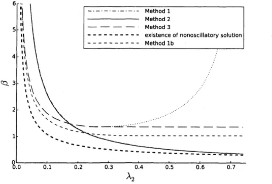
On the following graphs

we

illustrate these bounds

as

functions of$\lambda_{2}$

.

In order to allow both

variants of method of apriori bound, we will consider the linear case $p=2$. Thus Methods 1

and lb reﬀer tothe method ofapriorybound with comparisonto second order ordinary and delay

diﬀerentialequation, respectively. Further Methods 2 and 3 reﬀer tothe method of Riccatiequation

and comparison method. The dotted curvewhich branches oﬀthe curve for Method 3 denotes the

result ofcomparison method without considering the case $\eta\neq\sigma$ in Theorem 2, i.e. without the

$\min$_{operator in (24),} _{which is often considered in the literature.}

Observe, that if$b_{0}$ issmall, then estimate based on Method 1 is reasonably good,

but becomes

worse as $b_{0}$ increases. Note also that we obtain better results from Riccati method if

$\lambda_{2}$ is large.

On thecontrary, if$\lambda_{2}$ issmall,

better bound fortheoscillation constant $\beta$ canbe obtained fromthe

comparison _{method. Note also that the} _curves _{for Methods} lb and 3 end up with constant parts,

theother curves aredecreasing.

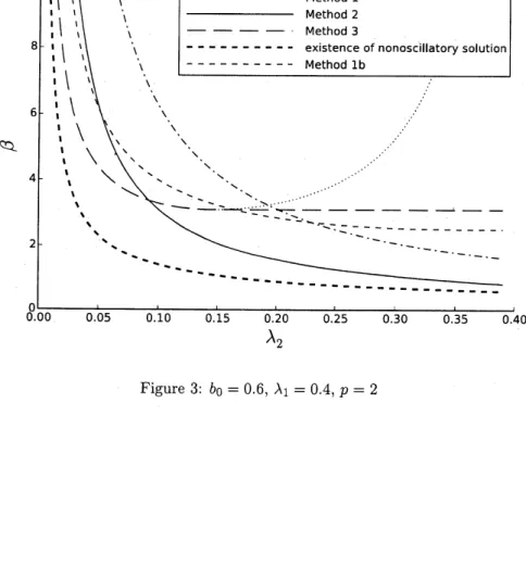
The following threepicturesdemonstrate the fact thatnomethod beats the otheronesand that

the mutual relationship of the obtainedcurves is rich. However thesepictures (aswell asexploring

more similar portaits) give thegeneral impression that

$\circ$ apriorymethod (Methods

1 and lb) wastes of$b_{0}$ is not small enough,

$\bullet$ forlarge delay(large

diﬀerence$t-\sigma(t)$,i.e. $\sigma(t)\ll t$) it ismoreconvenient touse_the_methods

based _{on Myshkis-type oscillation criteria for delay diﬀerential} _{equations, i.e.} _{Method lb} _(if

$b_{0}$ is small) and Method 3

$\bullet$ for small delay (small

diﬀerence $t-a(t)$) it is more convenient to use the methods based on

oscillation criteriaforordinarydiﬀerentialequations,i.e. Method 1 (if$b_{0}$issmall) andMethod

(10)

Figure 1: $b_{0}=0.1,$ $\lambda_{1}=0.75,$ _$p=2$, Method 1 almost coincides with Method 2,

(11)

o.oo

0.$05$ 0.$10$ _0.15 _0.20 $\lambda_{2}$

0.25 0.30 0.35

(12)

References

[1] R. P. Agarwal, M. Bohner, T. Li, Ch Zhang, Oscillationofsecond-order Emden-Fowler neutral

delaydiﬀerential equations, Ann. Mat. PuraAppl. (2014) 193, 1861-1875.

[2$|$ J. G. Dong, Oscillation behavior ofsecondorder nonlinearneutral diﬀerential equationswith

deviating arguments, Comp. Math. Appl. 59 (2010), 3710-3717.

[3] O. Do\v{s}l\’y, P.

\v{R}eh\’ak,

Half-Linear Diﬀerential Equations. North-Holland Mathematics Studies

202, Elsevier, 2005.

[4] B. Bacul\’ikov\’a, J. D\v{z}urina, Oscillation theorems for second-orderneutraldiﬀerential equations,

Comp. Math. Appl. 61 (2011), 94-99.

[5] B. Bacul\’ikov\’a, J. D\v{z}urina, Oscillation theorems for second-order nonlinear neutral diﬀerential

equations, Comp. Math. Appl. 62 (2011), 4472-4478.

[6] B. Bacul\’ikov\’a, T. Li, J. D\v{z}urina, Oscillation theorems for second order neutral diﬀerential

equations, E. J. Qualitative Theory of Diﬀ. Equ., No. 74 (2011), 1-13.

$[7|$ B. Bacul\’ikov\’a, T. Li, J. D\v{z}urina, Oscillation theorems for second-order superlinear neutral

diﬀerentialequations, Math. Slovaca63 No. 1 (2013), 123-134.

[8] S. Fi\v{s}narov\’a, R. Ma\v{r}\’ik, Oscillation ofhalf-lineardiﬀerentialequationswith delay, Abstr.Appl.

Anal. (2013), Article ID 583147, 1-6.

$[9|$ S. Fi\v{s}narov\’a, R. Ma\v{r}\’ik, On eventually positive solutions ofquasilinear second order neutral

diﬀerentialequations, Abstr. Appl. Anal. 2014 (2014), Article ID 818732, 1-11.

[10] S. Fi\v{s}narov\’a, R. Ma\v{r}\’ik, Oscillation criteria for neutral second-order half-linear diﬀerential

equations with applications to Euler type equations, Bound. Value Probl. 2014:83 (2014),

1-14.

[11] Z. Han, T. Li, S. Sun, W. Chen, Oscillation criteria for second-order nonlinear neutral delay

diﬀerentialequations, Adv. Diﬀerence Equ. (2010), Article ID 763278, 1-23.

[12] R.G.Koplatadze, Criteriaforthe oscillation ofsolutions ofdiﬀerentialinequalities and

second-orderequationswith retarded argument, (Russian) Tbiliss. Gos. Univ. Inst. Prikl. Mat. Trudy

17 (1986), 104-121.

[13] T. Li, Comparison theorems for second-order neutral diﬀerential equations of mixed $type_{\}}$

Electron. J. Diﬀ. Equ., Vol. 2010(2010), No. 167, 1-7.

[14] T. Li, Z. Han, Ch. Zhang, H. Li, Oscillation criteria for second-ordersuperlinear neutral

dif-ferentialequations, Abstr. Appl. Anal. (2011), Article ID 367541, 1-17.

[15] T.Li, Y. V. Rogovchenko, Ch. Zhang, Oscillationofsecondorder neutral diﬀerentialequations,

Funkcial. Ekvac. 56 (2013), 111-120.

[16] Z. Oplu\v{s}til, J.

\v{S}remr,

Onoscillations ofsolutions tosecond-order lineardelaydiﬀerential

(13)

[17] S. Sun,T. Li, Z. Han,H. Li,Oscillation theorems for secondorder quasilinear neutralfunctional

diﬀerential equations, Abstr. Appl. Anal. (2012), Article ID 819342, 1-17.

[18] M. Hasanbulli, Y. Rogovchenko, Oscillation criteria for second order nonlinear neutral

diﬀer-ential equations, Appl. Math. Comp. 215 (2010),4392-4399.

Department of Mathematics

Mendel University in Brno

Zem\v{e}d\v{e}lsk\’a 1

61300

Brno

CZECH REPUBLIC