Extra singularities of geometric solutions to
Monge-Amp\‘e
$\mathrm{r}\mathrm{e}$equations
of
three
variables.
Goo
ISHIKAWA
and Yoshinori
MACHIDA
$\text{ノ}\mathrm{E}^{\mathrm{I}\mathrm{I}}|\#|^{[]}|\mathrm{R}\triangleright$ $C4CA\cdot\Phi 1$
$1$
Introduction.
$/_{|\tau’)\mathrm{z}}^{/\mathit{4}}$
$\epsilon \mathit{4}_{/\backslash ^{\vee},\mathrm{C}_{\mathrm{t}\supset}^{\backslash },\prime}^{\mathrm{a}_{\mathcal{D}-\doteqdot\#,)}}.\cdot‘ \mathrm{o}\mathrm{L}$
In this survey article, we review recent results on singularities of solutions
to Monge-Amp\‘ere equations of two independent variables [12], and give the
generic classification for Monge-Amp\‘ere equations ofthree independent
vari-ables. Then we find the remarkable difference in generic singularities which
appear in the case of two variables and three variables. The details will be
given in the forthcoming paper.
Solutions to a Monge-Amp\‘ere equation
$\det(.\frac{\partial^{2}z}{\partial\prime r_{i}\partial x_{j}})_{1\leq i,j\leq n}=g(x_{1},x_{2},$
$\ldots,$$x_{n},$$z,$
$\frac{\partial z}{\partial x_{1}},$$\frac{\partial z}{\partial\tau_{2}}.$ $\cdots,$
$\frac{\partial z}{\partial x_{n}}.)$
for a function $z=z(x),$$x=(x_{1}, .\tau_{2}, \ldots x_{n})\rangle$
’ can be treated as a Legendrian
submanifold, a geometric solution, in the $(x, z,p=\partial z/\partial x)$ space satisfying
a condition due to the equation. Then the singularities of a solution are
regarded as Legendrian singularities; singularities of a geometric solution via
the Legendrian projection $(x, z,p)\mapsto(x, z)$.
The list of generic singularities of Legendrian projections of Legendrian
submanifolds (which are not necessarily geometric solutions) consists of the
cuspidaledge ($A_{2}$-singularity) and theswallowtail ($A_{3}$-singularity) inthe case
oftwo variables. See Figure 1.
In the case of three variables, the list consists of $A_{2},A_{3},$ $A_{4}$ and $D_{4^{-}}$
singularities. The $A_{4}$-singularity is called the butterfly. The $D_{4}$ singularities
are the pyramid (elliptic umbilic, $D_{4}^{-}$) and the purse (hyperbolic umbilic,
$D_{4}^{+})[4]$. Figures 2 and 3 illustrate the caustics, the loci of singularities in
Figure 1: the cuspidal edge (left) and the swallowtail (right)
Figure 2: Caustics of $A_{2},$ $A_{3}$ and $A_{4}$-singularities in the three space
In [12],
we
study on the singularities of solutions to the Monge-Amp\‘ere equation$\det$
(
$\frac{\frac{\partial^{d})f}{\partial x^{2}\partial^{2}f}}{\partial y\partial x}$ $\frac{\partial^{9}arrow f}{\partial_{\backslash }y,\frac{\partial^{2}fx\partial}{\partial y^{2}}})=c$,$c$ being a constant, the equation of improper affine spheres, and
$\det$
(
$\frac{\frac{\partial^{2}f}{\partial^{2}f\partial x^{2}}}{\partial y\partial\prime \mathrm{r}}$.
$\frac{\partial^{2}f}{\partial..y,\frac{\partial^{9}f\prime r\partial}{\partial y^{2}}})=c(1+(\frac{\partial f}{\partial x})^{2}+(\frac{\partial f}{\partial y})^{2})^{2}$ ,
the equation of surfaces with the constant Gaussian curvature. Then it is
shown that generic singularities of solutions to each equation are cuspidal
edges and swallowtails as in the case without an equation. Moreover, in the
case $c\neq 0$, also the list of generic singularities of dual surfaces turns to be
the same. To show the classification results, we used in [12] the criterion of
cuspidal edges and swallowtails established in [17].
We clarify our class of Monge-Amp\‘ereequations, Hessian Monge-Amp\‘ere
equations, recalling the formulation established in [13]. Then we generalise
the classification result in [12] to general Monge-Amp\‘ere equations in
\S 3.
Moreover, in the
case
of three variables, weannounce
that there appearextra singularities in generic solutions to a Monge-Amp\‘ere equation, other
than $A_{2},$ $A_{3},$ $A_{4},$ $D_{4}$-singularities in
\S 4.
Moreover in \S 5 we explain roughlythe method of generating families to show the classification results in this
paper.
In this paper, all manifolds and mappings are assumed to be ofclass $C^{\infty}$
unless otherwise stated.
2
Monge-Amp\‘ere
equations
with
Lagrangian
pairs.
In [13], we introduce a class of Monge-Amp\‘ere equations; Monge-Amp\‘ere
systems with aLagrangian pair. Consider $\mathrm{R}^{2n+1}$ with coordinates $(x, z,p)=$
$(x_{1}, x_{2}, \ldots,x_{n}, z,p_{1},p_{2}, \ldots,p_{\mathfrak{n}})$ and the contact form
on $\mathrm{R}^{2n+1}$. The contact distribution $D=\{\theta=0\}\subset T\mathrm{R}^{2n+1}$
has the
decom-position $D=D_{1}\oplus D_{2}$ into the pair of two Lagrangian sub-bundles
$D_{1}= \langle\frac{\partial}{\partial p_{1}},$ $\frac{\partial}{\partial p_{2}}$ $\ldots,$
$\frac{\partial}{\partial p_{n}}\rangle$
and
$D_{2}= \langle\frac{\partial}{\partial x_{1}}+p_{1^{\frac{\partial}{\partial z’}}}\frac{\partial}{\partial x_{2}}+p_{2^{\frac{\partial}{\partial z’}}}\ldots,$ $\frac{\partial}{\partial x_{n}}.+p_{n}\frac{\partial}{\partial z}\rangle$
for the symplectic form $d\theta$ on $D$. We call $(D_{1}, D_{2})$ a Lagrangian pair. Since
$D_{1},$$D_{2}$ are both integrable, we have the Legendrian double fibrations:
$\mathrm{R}^{2n+1}$
$\pi_{1}\swarrow$ $\searrow\pi_{2}$ $\mathrm{R}^{n+1}$ $\mathrm{R}^{n+1}$,
where $\pi_{1}(x, z,p)=(x, z)$ and $\pi_{2}(x, z,p)=(p, x\cdot p-z),$ $x \cdot p=\sum_{i=1}^{n}x_{i}p_{i}$,
are projections along $D_{1}$ and $D_{2}$ respectively.
In general, a differential system $\mathcal{M}$ on a contact manifold is
called a
Monge-Amp\‘ere system if $\mathcal{M}$ is locally generated by a contact form
$\theta$ and an
$n$-form $\omega([21][22])$.
In particular consider an $n$-form $\omega$ on $\mathrm{R}^{2n+1}$ of the form
$\omega=\omega_{1}-\omega_{2}$, $\omega_{1},$$\omega_{2}$ satisfying that $u\rfloor\omega_{1}=0$ for any $u\in D_{1},$ $v\rfloor\omega_{2}=0$ for any $v\in D_{2}$,
$\omega_{1}|D_{2}$ is a volume form on $D_{2}$, and that $\omega_{2}|D_{1}$ is a volume form on $D_{1}$.
Then the differential system generated by $\theta$ and
$\omega$ is called a Monge-Amp\‘ere
system with the $La_{\theta}ran_{\mathit{9}^{ian}}$ pair $(D_{1}, D_{2})$. Then
we
can take $\omega=\omega_{1}-\omega_{2}$with
$\omega_{1}=g(x, zp\})dx_{1}\wedge dx_{2}\wedge\cdots\wedge d.x_{n}$, $\omega_{2}=dp_{1}\wedge dp_{2}\wedge\cdots\wedge dp_{n}$,
for a non-vanishing function $\mathit{9}=g(x, z,p)$. Since $n$ and the function $g$
determine the system, we designate it by $\mathcal{M}(n,g)$. Note that we
assume
$g$ is
non-vanishing (on the domain we work on).
An immersed submanifold $L^{r\iota}$ in $(\mathrm{R}^{2n+1}, D)$ of
dimension $n$ is called
Leg-endrian if $\theta|_{L}=0$ for a contact form $\theta$, namely, if $L$
is
an
immersed integralsubmanifold to $D$. A Legendrian submanifold $L$ in $(\mathrm{R}^{2n+1}, D)$ is called
a
ge-ometric solutionto aMonge-Amp\‘ere system generated by $\theta$ and
$\omega$ if$(\theta|_{L}=0$
and) $\omega|_{L}=0$.
A function $z$ : $Uarrow \mathrm{R}$ on a domain $U$ of $\mathrm{R}^{n}$ induces a Legendrian
submanifold $L$ in $\mathrm{R}^{2n+1}$ by
Then $L$ is a geometric solution to $\mathcal{M}(n, g)$ if and only if $z$ is a classical
solution to the equation
$\det(.\frac{\partial^{2}z}{\partial x_{i}\partial x_{j}}.)_{1\leq i,j\leq n}=_{\mathit{9}}(x_{1},$ $\ldots,$$x_{n},$$z,$ $\frac{\partial z}{\partial x_{1}},$ $\ldots,$
$\frac{\partial z}{\partial\tau_{1}}.)$
We call this type ofequations Hessian $\Lambda fonge- Amp^{t}ere$ equations.
Note that a geometric solution $L$ in $\mathrm{R}^{2\mathrm{n}+1}$ gives a multi-valued classical
solution if $\pi_{1}|_{L}$ is immersive. A singular point of $L$
means
a non-immersivepoint of$\pi_{1}|_{L}$.
We denote by $\mathrm{H}\mathrm{e}\mathrm{s}\mathrm{s}(z)$ the Hessian determinant of$z=z(x_{1}, x_{2}, \ldots,x_{n})$.
Example 2.1 Consider theequation $\mathrm{H}\mathrm{e}\mathrm{s}\mathrm{s}(z)=c,$ $(c\neq 0)$ for improperaffine
spheres $z=z(x_{1}, \ldots, x_{n})$ of dirnension $n$. The corresponding Monge-Amp\‘ere
system $\mathcal{M}(n, c)$ to it is generated by the contact form $\theta=dz-p_{1}dx_{1}$-
-$p_{n}dx_{n}$ and Ca7 $=cdx_{1}\wedge dx_{2}\wedge\cdots\wedge dx_{n}-dp_{1}\wedge dp_{2}\wedge\cdots\wedge dp_{n}$.
Example 2.2 Theequation $K=c,$$(c\neq 0)$ for surfacesofconstant Gaussian
curvature is described by the Monge-Amp\‘ere system $\mathcal{M}(2, c(1+p_{1}^{2}+p_{2}^{2})^{2})$
generated by the contact form $\theta=dz-p_{1}dx_{1}-p_{2}dx_{2}$ and
$\omega=c(1+p_{1}^{2}+p_{2}^{2})^{2}dx_{1}\wedge dx_{2}-dp_{1}\wedge dp_{2}$.
By J\"orgens, Calabi and Pogorelov’s theorems, a global convex solution
$z$ : $\mathrm{R}^{n}arrow \mathrm{R}$ to the equation $\mathrm{H}\mathrm{e}\mathrm{s}\mathrm{s}(z)=c(c>0)$ is necessarily a quadratic
polynomial function. By Hilbert’s theorem, we see that there does not
ex-ist any complete surface satisfying
$K=c(c<0)$
. Alsowe
see, byLieb-$\mathrm{m}\mathrm{a}\mathrm{n}\mathrm{n}^{)}\mathrm{s}$ theorem, any complete surface with
$K=c(c>0)$
is a sphere.Therefore it is indispensable to study singularities of solutions to
Monge-Amp\‘ere equations. Then generic classification of singularities of
geomet-ric solutions to the corresponding Monge-Amp\‘ere systems provides one of
higher perspective beyond intuitive and analytic approaches to the solutions
to Monge-Amp\‘ere equations. Moreover we classify singularities of the
orig-inal solution $z=z(x_{1},x_{2}, \ldots, x_{n})$ as well as its Legendre transformation
$\tilde{z}=\sum_{i=1}^{n}p_{i}x_{i}-z=\sum_{i=1}^{n}\frac{\partial z}{\partial x_{i}}x_{i}-z$.
The geometric foundation
on
Monge-Amp\‘ere equations is given, forin-stance, in $[21][22][18][6][15][5]$. For related geometric studies on singularities
can
beseen
in $[9][20][17][14]$. For arelated analytic studyon
Monge-Amp\‘ereequations can be seen, for instance, in [10].
Lemma 2.3 Let $L\subset \mathrm{R}^{2n+1}$ be a geometric solution to a Monge-Amp\‘ere
system A4$(n, g)$
for
a non-vanishingfunction
$g$.
Then $\ell\in L$ is a $sin_{\mathit{9}}ul_{}ar$point
of
$\pi_{1}|_{L}$if
and onlyif
$\ell\in L$ is a singular pointof
$\pi_{2}|_{L}$.Proof:
Since $\theta|_{L}=0$, we see $\ell\in L$ is a singular point of $\pi_{1}|_{L}$ if and only if$dx_{1}\wedge dx_{2}\wedge\cdots\wedge d.x_{n}|_{L}=0$ at, $\ell$. Similarly, since
$\theta=-(d(\sum_{i=1}^{n}p_{i}x_{i}-z)-$
$\sum_{i=1}^{n}.x_{i}dp_{i})=0$ on $L$, we see $\ell\in L$ is a singular point of $\pi_{2}|_{L}$ if and only if
$dp_{1}\wedge dp_{2}\wedge\cdots\wedge dp_{n}|_{L}=0$ at $\ell$. Now
$\omega=g(x, z,p)dx_{1}\wedge dx_{2}\wedge\cdots\wedge dx_{n}-dp_{1}\wedge dp_{2}\wedge\cdots\wedge dp_{n}=0$
on
$L$, and $g(\ell)\neq 0$. Thuswe see
$dx_{1}\wedge dx_{2}\wedge\cdots\wedge dx_{n}|_{L}=0$ at $\ell$ if and$\mathrm{o}\mathrm{n}\mathrm{l}\mathrm{y}\square$
if$dp_{1}\wedge dp_{2}\wedge\cdots\wedge dp_{n}|L=0$ at $\ell$.
Also the following is fundamental:
Lemma 2.4 $\pi_{1*}|\mathrm{K}\mathrm{e}\mathrm{r}(\pi_{2}|_{L})_{*}$ is injective. Similarly $\pi_{2*}|\mathrm{K}\mathrm{e}\mathrm{r}(\pi_{1}|_{L})_{*}$ is
injec-tive.
Proof:
Since $(\pi_{1}, \pi_{2})$ : $\mathrm{R}^{2n+1}arrow \mathrm{R}^{n+1}\cross \mathrm{R}^{n+1}$ is an embedding, the restriction$\mathrm{e}\mathrm{a}\mathrm{s}\mathrm{i}1\mathrm{y}(\pi_{1}|_{L},.\pi_{2}|_{L})$
: $Larrow \mathrm{R}^{n+1}\cross \mathrm{R}^{n+1}$isan immersion. Therefore Lemma2.4
$\mathrm{f}\mathrm{o}\mathrm{l}\mathrm{l}\mathrm{o}\mathrm{w}\mathrm{s}\square$
3
Monge-Amp\‘ere equations
of
two variables.
The result in [12] is generalised to the following result:
Theorem 3.1 Let$g(x_{1}, x_{2}, z,p_{1},p_{2})$ be a non-vanishing analytic
function
ona domain
of
$\mathrm{R}^{5}$.
Then,for
generic geometric solutions to the Monge-Amp\‘eresystem $\mathcal{M}(2, g)$ corresponding to the equation
$\det(\frac{\partial^{2}z}{\partial_{X_{i}}\partial x_{j}})_{1\leq i,j\leq 2}=g(x_{1},$ $x_{2},$$z,$ $\frac{\partial z}{\partial x_{1}}.’\frac{\partial z}{\partial x_{2}})$ ,
the pair
of
$\pi_{1}$-Legendrian singularity and $\pi_{2}$-Legendrian singularity at anypoint is given exactly by the list:
$(A_{1}, A_{1}),$ $(A_{2}, A_{2}),$ $(A_{2}, A_{3}),$ $(A_{3}, A_{2})$.
All
four
cases actually appear in ageometric solution to $M(2, g)$ and theyare stable under smal,$l$perturbations
For a generic Legendrian submanifold $L^{9}arrow$ in $\mathrm{R}^{5},$ $\theta|_{L}=0$, we $\mathrm{h}a\mathrm{v}\mathrm{e}$ six
cases:
$(A_{1}, A_{1}),$ $(A_{1}, A_{2}),$ $(A_{1}, A_{3}),$ $(A_{2}, A_{1}),$ $(A_{9,\sim}, A_{2}),$ $(A_{3}, A_{1})$.
By Theorem 3.1, for a generic $L^{2}$ in $\mathrm{R}^{\overline{0}}$ with $\theta|_{L}=0,\omega|_{L}=0$, just
the cases $(A_{1}, A_{1}),$ $(A_{2}, A_{2})$ are realised as generic singularities of a
Monge-Amp\‘ereequation, and moreovertwocases $(A_{2}, A_{3}),$ $(A_{3}, A_{2})$ occurgenerically
as singularities of a Monge-Amp\‘ere equation, while they are not generic as
singularities of Legendrian immersions via the Legendrian double fibration.
The equation provides the essential restriction via Lemma 2.3.
Similarly as in [12], Theorem 3.1
can
be proved by using the criterionof [17]. Also the method of generating families can be applied; in the next
section, we show the outline of the method, in the case of three variables.
The method is applied equally to the case of two variables. We assume 9
is analytic in Theorem 3.1 and in Theorem 4.1 below. This is because we
use
the theorem of Cauchy-Kovalevskaya to guarantee the solvability of aninitial value problem.
4
Monge-Amp\‘ere
equations
of three
variables.
As is mentioned already in Introduction, it is known that the generic
Legen-drian singularities of three dimension are $A_{1}$, $A_{2)}A_{3},$ $A_{4},$$D_{4}^{+},$$D_{4}^{-}[4]$. However
we easily see that the generic singularities of geometric solutionsto a
Monge-Amp\‘eresystem with a Lagrangian pairof three variables never have thesame
list. Regardingwith the symmetry between$\pi_{1}$ and $\pi_{2}$, suppose they have the
same list, and suppose $\pi_{2}|_{L}$ is of type $D_{4}$ at $\ell\in L$ for a generic $L$ via both
$\pi_{1}$ and $\pi_{2}$. Then $\dim \mathrm{K}\mathrm{e}\mathrm{r}(\pi_{2}|_{L})_{*}=2$. Then, by Lemma 2.4, we have
$\pi_{1}|_{L}$ is
of rank 2 so it must be of type $A_{k}$. However, by Lemma 2.3, the singular
loci of $\pi_{1}|_{L}$ and $\pi_{2}|_{L}$ coincide. The singular locus of an $A_{k}$-singularity is
non-singular itself, On the other hand, the singular locus of a $D_{4}$-singularity
is a cone, which has a singularity. These lead a contradiction.
In the case ofthree variables, in fact we get the list
$A_{1},$ $A_{2},$ $A_{3},$ $A_{4},$$D_{4}^{+},$ $D_{4}^{-},$ $A_{3}(+$, -$)$, $A_{3}$(-, -)
ofgeneric singularities of geometric solutions.
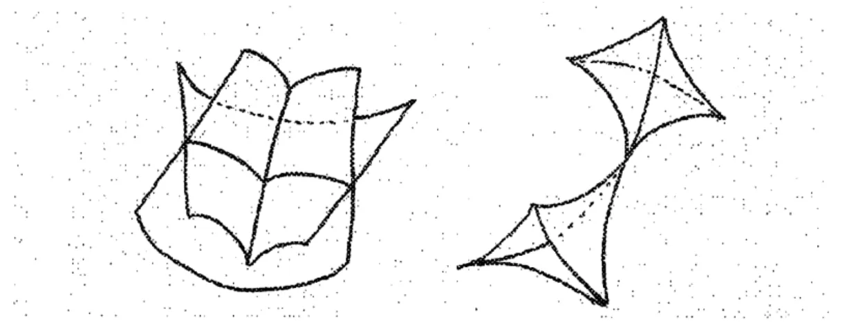
Thesingularitiesoftype $A_{3}(+$, -$)$ (“$\mathrm{c}\mathrm{u}\mathrm{s}\mathrm{p}\mathrm{i}\mathrm{d}\mathrm{a}\mathrm{l}$ cone”) and $A_{3}(-$,-$)$
(“cone-cone”) appear also as instantaneous singularities (of codimension one) in
wavefront evolutions $[1][26]$. The pictures ofthe caustics (the singular lociin
the $(x_{1},x_{2}, x_{3})$-space) corresponding to $A_{3}(+$, -$)$ and $A_{3}(-, -)$-singularities
are given in Figure 4. See also $[2][3]$.
Figure 4: Caustics of $A_{3}(+$, -$)$ and $A_{3}(-$,- $)$ in the three space
Theorem 4.1 Let $g(x_{1}, x_{2}, x_{3}, z,p_{1},p_{2},p_{3})$ be a
non-vanishin9
analyticfunc-tion on a domain
of
$\mathrm{R}^{7}$.$Then_{f}$
for
generic geometric solutions to theMonge-Amp\‘ere system $\mathcal{M}(3, g)$ corresponding to the equation
$\det(\frac{\partial^{2}z}{\partial x_{i}\partial x_{j}})_{1\leq i,j\leq 3}=g(x_{1},$ $x_{2},$$.x_{3},$ $z,$ $\frac{\partial z}{\partial x_{1}},$ $\frac{\partial z}{\partial x_{2}},$$\frac{\partial z}{\partial x_{3}})$ ,
the pair
of
$\pi_{1}$-Legendrian $sin_{\mathit{9}}ularity$ and $\pi_{2}$-Legendrian singularity at anypoint is given $exactl,y$ by the list:
$(A_{1}, A_{1}),$ $(A_{2}, A_{2}),$ $(A_{2}, A_{3}),$ $(A_{2}, A_{4}),$ $(A_{3}, A_{2}),$ $(A_{3}, A_{3}),$ $(A_{4}, A_{2})$,
$(A_{3}(+, -),$$D_{4}^{+}),$ $(A_{3}(-, -),$$D_{4}^{-}),$ $(D_{4}^{+}, A_{3}(+,-))$, and $(D_{4}^{-}, A_{3}(-,-))$.
All eleven cases actually appear in a geomebric solution to $\mathcal{M}(3, g)$ and
they
are
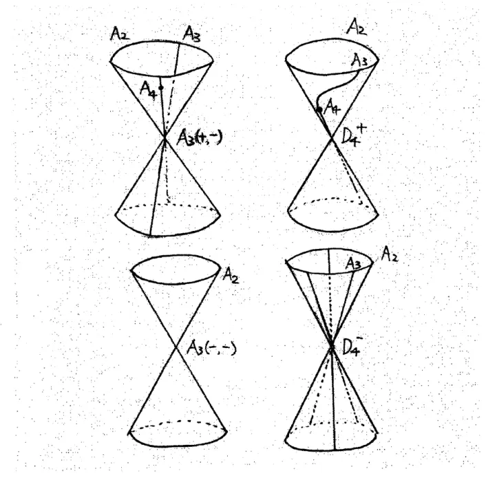
stable undersmallperturbations amonggeometric solutions to$\mathcal{M}(3,g)$.The stratiPcations of $L$ by singularities of double Legendrian fibrations
are illustrated as Figure 5.
Note that, by Theorem 4.1, each ofthesesingularitiesappears
as a
genericand stabl,$e$ singularity of a Monge-Amp\‘ere equation. Also note that another
singularity $A_{3}(+, +)$ ($‘ {}^{\mathrm{t}}\mathrm{t}\mathrm{h}\mathrm{e}$
birth of flying saucer” $[2][3]$) does not appear
generically in solutions ofa Monge-Amp\‘ere equation.
5
Solutions
to generalised Chynoweth-Sewell
equations.
. .
..
.
Figure 5: Stratifications by double Legendrian fibrations of a geometric
Let $L^{3}\subset \mathrm{R}^{7}$ be a geometric solution to $\mathrm{H}\mathrm{e}\mathrm{s}\mathrm{s}(z)=c,$ $(c\neq 0)$. Suppose $\pi_{1}|_{L}$ is of rank 2 and $\pi_{2}|L$ is of rank 1 at a point $\ell$ on $L$. Then we can set $L$ :
$x_{1}=u,$ $x_{2}=v,$ $x_{3}=- \frac{\partial h}{\partial w},$ $z=h- \frac{\partial h}{\partial w}w,$ $p_{1}= \frac{\partial h}{\partial u},$ $p_{2}= \frac{\partial h}{\partial v},$
$p_{3}=w$,
foraparameter $(u, v, w)$ centred at $\ell$andagenerating function $h=h(u, v, w)$.
Then the
anal:
sis on singularities ofsolutions to the equation $\mathrm{H}\mathrm{e}\mathrm{s}\mathrm{s}(z)=c$isreduced that of the equation
$c \frac{\partial^{2}h}{\partial w^{2}}+$
$\frac{\partial^{2}h}{\partial u^{2}}$ $\frac{\partial^{2}h}{\partial u\partial v}$
$\frac{\partial^{2}h}{\partial v\partial u}$ $\frac{\partial^{2}h}{\partial v^{2}}$
$=0,$ $\cdots\cdots(\mathrm{C}\mathrm{S})$
for $h=h(u, v, w)$
.
The equation $(\mathrm{C}\mathrm{S})$ is called a Chynoweth-Sewell equation[5] and appears in meteorology [8].
In general, for the equation
$\mathrm{H}\mathrm{e}\mathrm{s}\mathrm{s}(z)=g(x, z,p)$,
we reduce our classification problem to the analysis ofclassical solutions to
$\Gamma(u, v, w)\frac{\partial^{2}h}{\partial w^{2}}+$
$\frac{\partial^{2}h}{\partial u^{2}}$
$\frac{\partial^{2}h}{\partial v\partial u}$
$\frac{\partial^{2}h}{\partial u\partial v}$
$\frac{\partial^{2}h}{\partial v^{2}}$
$=0,$ $\cdots\cdots$ (GCS)
a generalised Chynoweth-Sewell $equat_{\text{ノ}}ion$, for a non-vanishing function $\Gamma$, by
setting
$\Gamma(u, v, w)=g(u, v, \frac{\partial h}{\partial w}, w\frac{\partial h}{\partial w}-h, -\frac{\partial h}{\partial u}, -\frac{\partial h}{\partial v}, w)$.
The generating family for the projection $\pi_{1}$ of $L$ is given by
$F(w;x_{1},x_{2}, x_{3}, z)=z-x_{3}w+h(x_{1}, x_{2}, w)$.
This means that $L$ is given by
$L=\{(x_{1},x_{2}, .x_{3}, z,p_{1},p_{2},p_{3})|F=0,$ $\frac{\partial F}{\partial w}=0,p_{i}=\frac{\partial F}{\partial x_{i}}$ for some $w\}$ .
On the other hand, the generating family for the projection $\pi_{2}$ of $L$ is
given by
This means that$L$ is given by
$L= \{(x_{1)}x_{2}, x_{3}.\tilde{z},p_{1},p_{2},p_{3})|G=\frac{\partial G}{\partial u}=\frac{\partial G}{\partial v}=0,$ $x_{i}= \frac{\partial G}{\partial p_{i}}$ for some $(u, v)\}$
Note that $\tilde{z}=x_{1}p_{1}+_{\backslash }x_{2}p_{2}+x_{3}p_{3}-z$.
Solving the initial value problem of (GCS), we get the general form of $h$
and thus $F$ and $G$.
The initial value problem for $h(u, v, w)$ of (GCS) is solved for given
$\varphi(u, v)=h(u, v, 0))\psi(u, v)=\frac{\partial h}{\partial w}(u, v, 0)$.
We see $F(w;0,0,0, \mathrm{O})=h(\mathrm{O}, 0, w)$ , and
$\frac{\partial F}{\partial z}(w;0,0,0,0)$ $=$ 1,
$\frac{\partial F}{\partial x_{2}}(w;0,0,0,0)$ $=$ $\frac{\partial h}{\partial v}(0,0, w)\}$
Suppose
$\frac{\partial F}{\partial x_{1}}(w;0,0,0,0)$ $=$ $\frac{\partial h}{\partial u}(0,0, w)$,
$\frac{\partial F}{\partial x_{3}}(w;0,0,0,0)$ $=$ $w$.
$\frac{\partial^{2}h}{\partial w^{2}}(0,0,0)=0,$ $\frac{\partial^{3}h}{\partial w^{3}}(0,0,0)=0,$$\frac{\partial^{4}h}{\partial w^{4}}(0,0,0)\neq 0$.
Then $F$ is a versal unfolding of $F(w;0,0,0,0)$ if and only if
1,$\frac{\partial h}{\partial u}(0,0, w),$ $\frac{\partial h}{\partial v}(0,0, w),$$w$
form a generator ofthe quotient vector space
$Q= \frac{\mathrm{R}[[w]]}{\langle F(w;0,0,0,0),\frac{\partial F}{\partial w}(w\cdot 0,0,0,0))\rangle_{\mathrm{R}[[w]]}}$.
See [4]. This condition is equivalent to that
$\frac{\partial^{3}h}{\partial w^{2}\partial u}(0,0,0)\neq 0,$ or $\frac{\partial^{3}h}{\partial w^{2}\partial v}(0,0,0)\neq 0$.
Recall that $\pi_{2}|_{L}$ is given by
$(\tilde{z},p_{1},p_{2}.p_{3})=(\tilde{z}(u,v),$$\frac{\partial h}{\partial u},$ $\frac{\partial h}{\partial v},$$u))$,
with $d\tilde{z}=x_{1}dp_{1}+x_{2}dp_{2}+x_{3}dp_{3}$. Since $\pi_{2}|_{L}$ is of rank 1 at $\ell\in L$, we have
By the equation (GCS) and t,h$a\mathrm{t}_{1}\Gamma(0,0,0)\neq 0$, we see
$\frac{\partial^{3}h}{\partial w^{2}\partial u}(0,0,0)=0,$ $\frac{\partial^{3}h}{\partial w^{2}\partial v}(0,0,0)=0$.
Thus we see the singularity of$\pi_{1}|_{L}$ at $L$ is ofcorank 1 but never of $A_{k}$-type.
In fact we get the extra singularities $A_{3}(+$, - $)$ and $A_{3}(-$, -$)$.
Example 5.1 Let consider the equation $\mathrm{H}\mathrm{e}\mathrm{s}\mathrm{s}(z)=1$ of three variables.
Then
$h(u, v, w)$ $=$ $\frac{1}{6}u^{3}+\frac{1}{2}uv^{2}+uvw+\frac{1}{2}v^{2}w-\frac{1}{2}(u^{2}-v^{2})w^{2}-\frac{1}{6}(u-2v)w^{3}$
$+ \frac{1}{12}w^{4}+\frac{1}{20}w^{5}+\frac{1}{30}w^{\mathrm{b}^{\neg}}$
give a geometric solution $L^{3}\subset \mathrm{R}^{7}$ with $\pi_{1}|_{L}$ is oftype $A_{3}(+$, - $)$ and $\pi_{2}|_{L}$ is
oftype $D_{4}^{+}$ at $\mathrm{O}\in \mathrm{R}^{7}$.
References
[1] V.I. Arnol’d, Wavefrontevolution andequivariantMorse lemma, Comm.Pure Appl.
Math., 39-6 (1976), 557-582.
[2] V.I. Arnol’d, Evolution ofsingularit\’ies ofpotentialflows in collision-free media and
the metamorphosis of caustics in three-dimensional space, Journalof Soviet Math.,
32 (1986), 229-258.
[3] V.I. Arnol’d, Catastrophe Theow, Springer-Verlag.
[4] V.I.Arnol’d, S.M. Gusein-Zade, A.N.Varchenko, SingularitiesofDifferentiable Maps
I, Birkh\"auser, 1985.
[5] B.Banos, Nondegenerate Monge-Amp\‘ere stretctures in dimension 6, Letterin Math-ematical Physics 62 (2002), 1-15.
[6] R. Bryant, P. Griffiths, D. Grossman, Exterior Differential Systems and Euler-Lagrange PartialDifferential Equation, The University of Chicago Press (2003).
[7] E. Calabi, Improper affine hyperspheres of convex type and a generalizat\’ion of a
theorem by K. Jorgens, Michigan Math. J., 5 (1958), 105-126.
[8] S. Chynoweth, M.J. Sewell, Dual variables in semi-geostrophic theow, Proc. Roy.
Soc. London Ser. A 424 (1989), 155-186.
[9] L. Ferrer, A. Mart\’inez, F. Mil\’an, An extension of a theorem by K. J\"orgens and a
maximum principle at infinity for parabolic affine spheres, Math. Z., 230 (1999),
471-486.
[10] C.E. Guti\’errez, The Monge-Amp\‘ere Equations, Progress in Nonlinear Diff. Eq. and TheirAppl. 44 (2001).
[11] D.Hilbert, UeberFl\"ahen (jonconstanter GaussscherKrummung, Rans.Amer.Math.
Soc., 2-1 (1901), 87-99.
[12] G. IshikawaandY. Machida, Singularities ofimproper $affi_{}ne$ spheres and surfaces of
constant Gaussian $curvature_{\rangle}$ International J. Math. 17-3 (2006), 1-25.
[13] G. Ishikawa and Y. Machida, Monge-Amp\‘ere systems with Lagrangian pairs, in
preparation.
[14] G. Ishikawa and T. Morimoto, Solutionsurfaces ofthe Monge-Amp\‘ere equation, Dif-ferential Geometry and its Applications, 14 (2001), 113-124.
[15] T.A.IveyandJ.M.Landsberg, Cartanforbeginners: differentialgeometry viamoving
frames and exterior differential systems, Amer. Math. Soc., (2003).
[16] K. J\"orgens, \"Uber die $L\ddot{\mathit{0}}s\cdot ungen$ der Differentidgleichung rt–s2 $=1_{f}$ Math. Ann.,
127 (1954), 130-134.
[17] M. Kokubu, W. Rossman, K. Saji, M. Umehara, K. Yamada, Singularities of flat
fronts in$h\varphi erbolic\mathit{3}$-space, to appear in Pacific J. Math..
[18] V.V.Lychagin, V.N. Rubtsov, I.V. Chekalov, A classification ofMonge-Ampere
equa-tions, Ann. Sci. \‘Ec. Norm. Sup., 26 (1993), 281-308.
[19] Y. Machida and T. Morimoto, On decomposable Monge-Amp\‘ere equations,
Lobachevskii J. Math. 3 (1999), 185-196.
[20] A. Mart\’inez, Improper affine maps, Math. Z., 249 (2005), 755-766.
[21] T. Morimoto, Lag\’eom\’etrie des \’equations de Monge-Amp\‘ere, C. R. Acad. Sci. Paris,
289 (1979), 25-28.
[22] T. Morimoto, Monge-Amp\‘ere equations viewed from contact geometry, in Banach CenterPublicationsvol.39 “SymplecticSingularitiesandGeometryof GaugeFields” , (1998), pp. 105-120.
[23] K. Nomizu andT. Sasaki, Affme differentialgeometry, Cambridgebacts in Math., 111, CambridgeUniv. Press (1994).
[24] B. O’Neill, Elementary Differential Ceometry, Academic Press (1966).
[25] A.V. Pogorelov, Onthe improper convex affine hypersurfaces, Geometriae Dedicata, 1 (1972), 33-46.
[26] V.M. Zakalyukin, Reconstructions ofwavefrontsdependingon oneparameter, Funct. Anal. Appl., 10-2 (1976), 139-140.
Goo ISHIKAWA
Department ofMathematics, $\mathrm{H}\mathrm{o}\mathrm{k}\mathrm{l}\sigma \mathrm{a}\mathrm{i}\mathrm{d}\mathrm{o}$University, Sapporo 060-0810, JAPAN.
Yoshinori MACHIDA
Numazu College ofTechnology, 3600 Ooka, Numazu-shi, Shizuoka, 410-8501,