On the variance-stabilizing multivariate nonparametric regression estimation (Statistical Experiment and Its Related Topics)

On

the variance-stabilizing

multivariate

nonparametric

regression

estimation

Kiheiji

NISHIDA

and Yuichiro

J.

KANAZAWA

1

1

Introduction

The objective of this paper is to show the idea of the nonpara,metric

regres-sion estimator that produces constant estimator variance over all values of

the regressor va,riable. _{To a,ccomplish the purpose, we introduce the} varia,ble

bandwidth matrix based on a,symptotic considera,tions _{chosen so as to}

cor-rect heteroscedasticity, employingthe sa,me principle of the Aitken estima,tor

in linea,$r$ regression. We call the bandwidth matrix for this objective the

variance-sta,bilizing (henceforth VS) bandwidth matrix.

As past studies for theVS bandwidth, we know that Fanand Gijbel (1992)

introduced the idea of the VS bandwidth for the univariate local linear

esti-mator. However, they did not investigatethe VS bandwidth in detail because

thepaper was aimed at studying the variable bandwidth that minimizes mean

squared error (MSE). In contrast to this, Nishida and Kanazawa (2009, 2010)

lKiheiji NISHIDA is a student at the Graduate School of Systems and Information

Engineering, University of Tsukuba. Yuichiro J. KANAZAWA is Professor ofStatistics at

theGraduate Schoolof Systems and Information Engineering, University of Tsukuba,

1-1-1 Ten-noh-dai, Tsukuba, Ibaraki 305-8573, Japan. Correspondence concerning this article

should be addressed to Kiheiji NISHIDA. His e-mail address is [email protected].

This research is supported in part by the Grant-in-Aid for Scientific Research (C)(2)

$]2680310,$ $(C)(2)$ 16510103 and (B) 20310081 from the Japan Society for the Promotion

introduced the VS bandwidth for the univariate Nadaraya-Watson

(hence-forth NW) estimator and compared it to the Mean Integrated Squared Error

(MISE) minimizingfixed bandwidth in terms of global and local performance.

These two studies focus on univariate nonparametric regression estimators.

In the light of these two studies, we introduce the VS bandwidth matrix

for themultivariate NWestimator. In section 2, we show the brief summaries

of the multivariate NW estimator to know the principle of how the

VS

band-width matrix is introduced. In section 3, we introduce the VS bandwidth

matrix for the multivariate NW estimator. In each subsection of section 2,

we show the performance of the univa,riate a,nd _the biva,riate _{VS regression}

estimators. We also show the estimating procedure of the VS bandwidth

matrix in the univariate case. In section 4, we give concluding remark.

2

Summaries

of the

multivariate NW

estima-tor

2.1

Basic

setup

Let us consider a $p+1$ row vector $(X_{i0}, \ldots, X_{i(p-1)}, Y_{i})$ of random variables.

We assume $x_{i}$. $=(x_{i0}, \ldots, x_{i(p-1)}),$ $i=1,$ $\ldots,$$n$, are the realizations of random

explanatory vector $X_{i}$. $=(X_{i0}, \ldots, X_{i(p-1)})$, i.i.d. with respect to $i$ and whose

joint density function is denoted a,s $fx_{i}.(x_{i}.)$

on

support $I^{p}\in R^{p}$

.

The $n$

sample realizations of $(X_{i0}, \ldots, X_{i(p-I)})$ can be written in matrix form as

$(\begin{array}{lll}x_{\prime l0} \cdots x_{1(p-1)}| \ddots |x_{n0} \cdots x_{n(p-1)}\end{array})$

and we define the ith column of the matrix in (2.1) as $x_{i}$

.

We assume that

with the kth variable$X_{k},$ $j\neq k$

.

We assume that the response $Y_{i},$ $i=1,$ $\ldots,$$n$,

is influenced by the corresponding explana,tory vector $X_{7}\cdot$. in the form of

$m(X_{i}.)$ and the disturbance $U_{i}$ as

$Y_{i}=m(X_{i}.)+U_{i}$, (2.1)

where $m(\cdot)$ is _$m$ : $R^{p}arrow R$ function of the $X_{i}.$

.

The $U_{i}|X_{i}.’ s,$ $i=1,$

$\ldots,$$n$,

are ra,ndom _{variables independent with respect to} $i$, and assumed to be

in-dependent of $X_{j}.,$ $i\neq j$

.

We additionally a,ssume the first two conditional

moments of $U_{i}|X_{i}$. are

$E_{U_{i}|X_{i}}$_. $[U_{i}|X_{i}$. $=x_{i}.]=0$, (2.2)

$E_{U_{i}|X_{*}}$. $[U_{i}^{2}|X_{i}=x_{i}.]=\sigma^{2}(x_{i}.)$

.

Then, from the assumptions (2.1) and (2.2), we obtain

$m(x_{i}.)=E_{Y_{i}|X_{i}}$_. $[Y_{i}|X_{i}$. $= x_{i}.]=\int y_{i}f_{Y_{i}|X_{i}}.(y_{i}|x_{i}.)dy_{i}$

$= \frac{\int y_{i}f_{X_{i},Y_{i}}.(x_{i}.,y_{i})dy_{i}}{f_{X_{i}}(x_{i}.)}$,

where $f_{X;.,Y_{i}}(x_{i}., y_{i})$ is the multivariate density function of $(X_{i}., Y_{i}).$

Replac-ing unknown density function $f_{X_{i}.,y}(x_{i}., y_{i})$ and $f_{X_{i}}.(x_{i}.)$ with their

estima-tor $\overline{f_{X_{i}.,Y_{i}}}(x_{i}., y_{i})and.\overline{f_{X_{i}}.}(R,\cdot.)$ , we obtain thenonpa,rametric estimator $\hat{m}(x_{i}.)$

written as

$\hat{m}(x_{i}.)=\frac{\int y_{?:}\overline{f_{X_{*},Y}\dot{..}}(x_{i}.,y_{7}:)dy_{i,}}{\overline{f_{X_{*}}.}(x_{i}.)}$

.

(2.3)

In estimating the denominator of (2.3), we employ the multivariate kernel

density estimator with $pdimensi_{ona}J$ kernel function $K_{X}(x)$ at any point

$x=(x_{0}, \ldots, x_{(p-1)})$ on $I^{p}\in R^{p}$ and with multivariate symmetric bandwidth

matrix,

$H_{X}=(\begin{array}{lll}h_{00} \cdots h_{0(p-1)}| \ddots |h_{0(p-1)} h_{(p-l)(p-1)}\end{array}),$ $h_{00}>0,$

written as

$\overline{f_{H_{X}}}(x)=\frac{1}{n|H_{X}|}\sum_{i=1}^{n}K_{X}(H_{\overline{x}}^{1}(x-x\cdot.))$

.

(2.5)

Similarly, in estimating the numerator of (2.3), let $K_{X,Y}(x, y)$ be $(p+1)-$

dimensional kernel function at the point

$(x, y)=(xx, y)$

, and $H_{X,Y}$

be the $(p+1)\cross(p+1)$ dimensional symmetric smoothing _{parameter matrix,}

$H_{X,Y}=(h_{0(p-1)}...h_{(p-1)(p-1)}h_{(p-1)y_{/}}h_{0y}.\cdot h_{(p-1)y}h_{yy}h_{00}...\cdot\cdot.h_{0(p-1)}h_{0y^{\backslash }}$ $=(\begin{array}{ll}H_{X} h_{y}^{T}h_{y} h_{yy}\end{array})$ ,

where $h_{y}=(h_{0y}, \ldots, h_{(p-1)y})$

.

With this notation, $(p+1)$ dimensional kernel

density estimator that appears in the numerator of (2.3) is written as

$\overline{f_{H_{X,Y}}}(x, y)=\frac{1}{n|H_{X,Y}|}\sum_{i=1}^{n}K_{X,Y}(H_{\overline{X}^{1}Y}(x-x_{i}.,y-Y_{i}))$

.

(2.6)

Ifwe additionally assume that the kernel $K_{X,Y}(x, y)$ is multiplicativein terms

of X and $Y$, the smoothing parameter matrix is written as

$H_{X,Y}=(\begin{array}{ll}H_{X} 00 h_{yy}\end{array})$ , $|H_{X,Y}|=|H_{X}|h_{yy}$

and the numerator of (2.3) is rewritten by the symmetry of the kernel as

$\int\frac{y}{n|H_{X,Y}|}\sum_{i=1}^{n}Is_{X,Y}^{r}(H_{\overline{X}^{1}Y}(x-x_{i}., y-Y_{i}))dy$

$= \frac{1}{n|H_{X}|h_{yy}}\sum_{i=1}^{n}\int yK_{X}(H_{\overline{X}}^{1}(x-x_{i}.))Is_{Y}’(\frac{y-Y_{i}}{h_{yy}})dy$

$= \frac{1}{n|H_{X}|}\sum_{i=1}^{n}I\iota_{X}^{\nearrow}(H_{\overline{x}}^{1}(x-x_{i}.))Y_{i}$

.

(2.7)

Substituting the numerator and the $denominator$ in _{(2.3) respectively for}

(2.5) and (2.7), the multivariate NW estimator at the point $x$ is rewritten as

$\overline{m_{H_{X}}}(x)=\frac{\sum_{i=1}^{n}K_{X}(H_{\overline{x}}^{1}(x-x_{i}.).)Y_{i}}{\sum_{i=1}^{n}K_{X}(H_{\overline{x}}^{1}(x-x_{i}))}$

.

(For univaria,te _{ca荅se, Nada,raya 1964, 1965, 1970; Watson 1964; Wa,tson and}

Lea,dbetter _{1964. For multivariate ca,se, e.g. H\"ardle 2004). We write the}

kernel function $It_{X}’(x)$ a,s $K(x)$ for brevity.

2.2

A

restriction

on multivariate

bandwidth

matrix

We see the role of the off-diagonal elements of the bandwidth matrix in (2.4)

in kernel density estimation. Observe the multiva,riate _{gaussian kernel,}

$K( H_{\overline{x}}^{1}x)=\frac{1}{2\pi|H_{X}|}\exp[-\frac{1}{2}x(H_{\overline{x}}^{1})^{2}x^{T}]$ ,

and we find that $H_{X}^{2}$ corresponds to the variance covariance matrix $\Sigma$ of

the normal distribution. This means that the off-diagonal elements of the

bandwidth matrix $H_{X}$ in (2.4) reflect the correlation between the variables

in kernel function because the off-diagonal elements of $H_{x}^{2}$ are zero if _{$h_{(k)(j)}$},

$k\neq j$, are all set to be zero. This property is true of the symmetric kernel

functions defined by the quadratic form $x(H_{\overline{X}}^{1})^{2}x^{T}$ other than Ga,ussian.

Considering this property with the $0ff-diagona_{1}1$ elements of bandwidth

ma,trix _{in (2.4), we notice that it is better to employ a full bandwidth} $ma_{t}trix$

for kernel density estimation ifit is considered that

X.;

is correlated with $X_{j}$

.

In this point, Wand and Jones (1993) demonstrated in the bivariate density

estimation situation that MISE ofthe kernel densityestimator is deteriorated

$\overline{\overline{\rho 0.00.30.60.91.0}}$

the ratio (2.8) 1.00 0.93 0.74 0.37 0.00

Table 1: The ratio (2.8) for different values of correlation coefficient $\rho$ from

Wand and Jones (1993).

paper, they derived the theoretical

AMISE

of the bivariate kernel density

estimatorfor the bivariate normal distribution with its correlation coefficient

$p$

.

They also calculated the ratio,

$[ \frac{\inf_{H\in H_{full}}AMISE(H)}{\inf_{H\in H_{diag}}AMISE(H)}]^{\frac{3}{2}}=[\frac{2(1-\rho^{2})}{\rho^{2}+2}]^{\frac{1}{2}}$ , (2.8)

for different values of $\rho$, where $H_{diag}$ and $H_{full}$ are respectively the classes

of the bivariate diagonal and the bivariatefull bandwidth matrix. This ratio

can be interpreted as the costs from not using full bandwidth matrix for the

correlated data in kernel density estimation. The result in table 1 indicates

that there surely exist the costs.

However, when we employ a full bandwidth matrix in (2.4), the number

of parameters to be estimated is $p(p+1)/2$

.

_{If we take the curse of}

dimen-sionality into consideration, this is too many. To reduce the number of

pa-rameters to be estimated, the sphering approa,ch, as in e.g. Fukunaga (1972)

or Wand and Jones (1993), is available ifit is probable that $X_{i}$. is distributed

as normal distribution with variance covariance matrix $\Sigma$

.

That is, _{$1inea_{t}rly$}

transforming the data so that the sample variance covariance matrix is

diag-onal, we compute the density by the diagonal bandwidth matrix and finally

retransform the estimated pdfback to the original scale. In the following, we

assume that the data is approximately distributed as normal and the

spher-ing approach is available. Then we can sea,rch _{for the form of VS bandwidth}

2.3

On the

conventional bandwidth

matrices

Under the assumption of the dia,gona,1 bandwidth ma,trix, the bias and the

variance of the multivariate NW estimator are derived at every point $x$ (e.g.

H\"ardle2004) under the standardset ofassumptions on appendix A. The bias so obtained is

$E_{Y,X}[\overline{m_{H_{X}}}(x)]-m(x)$

$= \frac{\mu_{2}(I_{1_{X}^{\nearrow}})}{2f_{X}(x)}[2(\nabla m(x))^{T}H_{X}H_{X}^{T}\nabla f_{X}(x)+f_{X}(x)tr [H_{X}^{T}\nabla^{2}m(x)H_{X}]]+o(1)$,

where

$\nabla f_{X}(x)=(\begin{array}{l}\frac{\partial fx,(x)}{\partial_{T}o}|\frac{\partial fx(x)}{\partial x_{p-l}}\end{array}),$$\nabla^{2}f_{X}(x)=(\begin{array}{lll}\frac{\partial^{2}fx(x)}{\partial x\partial x} \cdots \frac{\partial^{2}fx(x)}{\partial xo\partial x_{p-1}}| \ddots |\frac{\partial^{2}fx(x)}{\partial r_{\prime\rho-]}\partial xo} \cdots \frac{\partial^{2}fx(x)}{\partial\tau_{p-]}\partial x_{\rho-1}}\end{array})$ ,

and

$\mu_{2}(It_{X}^{\nearrow})=\int\cdots\int tt^{T}K(t)dt$ and $t=(t_{0}, \ldots, t_{p-1})$

.

Simila,rly, the $variance$ so obta,ined _is

$V_{Y,X}[ \overline{m_{H_{X}}}(x)]=\frac{1}{n|H_{X}|}\cdot\frac{\sigma^{2}(x)}{f_{X}(x)}[\int\cdots\int K^{2}(t)dt]+o(1)$

.

(2.9)

When $h_{m}=h_{11}=\cdots=h_{(p-1)(p-1)}$, we can obtain the asymptotic MISE

(AMISE) and derive the $diagona1$ fixed bandwidth matrix that balances the

leading terms of the integrated variance and the integrated bia,$s$ squared

written as

$H_{f^{ixed}}=[\frac{[\int\cdots\int K^{2}(t)dt][\int\cdots\int\sigma^{2}(x)dx]}{\mu_{2}^{2}(K)T_{fixed}}]^{\frac{1}{p+4}}p^{\frac{1}{p+4}}\cdot n^{-\frac{1}{p+4}}\cdot I_{p},(2.10)$

where

and

$\alpha_{i}(x)=2(\frac{\partial m(x)}{\partial_{X_{i}}})(\frac{\partial f_{X}(x)}{\partial_{X_{i}}})+f_{X}(x)(\frac{\partial^{2}m(x)}{\partial_{X_{i}^{2}}}),$$i=0,$ _{$\cdots p-1$}

.

Hence the AMISE minimized by (2.10) is

$(p^{\overline{p}}+4- \lrcorner i+\frac{p^{\frac{4}{p+4}}}{4})[\frac{[\int\cdots\int K^{2}(t)dt]^{\frac{4}{p+4}}[\int\cdots\int\sigma^{2}(x)dx]^{\frac{4}{\rho+4}}}{[\mu_{2}^{2}(K)]^{-1}\overline{p}+\overline{4}[T_{fixed}]^{-R}\overline{p}+\overline{4}}]$

.

$n^{-\frac{4}{P+4}}$

.

In the same ma,nner _{to the} fixed one in _(2.10), the variable bandwidth

matrix that minimizes mean squared error MSE defined at each $x$ can be

obtained a,s

$H_{var}(x)=[\frac{[\int\cdots\int A^{\nearrow 2}(t)dt]\sigma^{2}(x)f_{X}(x)}{\mu_{2}^{2}(K)[\sum_{i=0}^{p-1}\alpha_{i}(x)]^{2}}]^{\frac{1}{\rho+4}}p^{\frac{1}{\rho+4}}$

.

$n^{-\frac{1}{p+4}}$

.

_{$I_{p}$}

and the AMISE so obtained by using (2.12) is

$(p^{\frac{-p}{\rho+4}}+ \frac{p^{\frac{4}{P+4}}}{4})[\frac{[\int\cdots\int K^{2}(t)dt]^{\frac{4}{\rho+4}}T_{var}}{[\mu_{2}^{2}(K)]^{-L}\overline{\rho}+\overline{4}}]\cdot n^{-\frac{4}{P+4}}$ ,

where

$T_{var}= \int\cdots\int[\sigma^{2}(x)]^{\frac{4}{p+4}}[\frac{1}{f_{X}(x)}[\sum_{i=0}^{p-1}\alpha_{i}(x)]^{2}]^{\overline{\rho}+\overline{4}}dxR$

.

When $h_{m}=h_{11}=\cdots=h_{(p-1)(p-1)}$ does not necessarily hold, it is difficult

to generalize both the fixed and the varia,ble _bandwidth ma,trices.

2.4

The

problem with

the

variance

of the

multivariate

NW

estimator

Weadderessthe problem with thevariance ofthe NW estimator. The leading

Both $fx(x)$ and $\sigma^{2}(x)$ are very unlikely to be uniform across different _$x$ in

general. As a result, variances of the NW estima,tor _{at different points} $x_{1}$

and $x_{2}$ differ in general unless properly controlled by the bandwidth ma,trix

$H_{X}$

.

As examples of the heterosceda,sticity of the NW estimator‘s variance,

see Nishida and Kanazawa (2009, 2010).

3

Introduction

of the

multivariate

VS

band-width

matrix

We consider the form of the bandwidth matrix that counters

heteroscedastic-ity. Employing the same principle oftheAitken estimator in linear regression,

we propose the VS bandwidth matrix at the point $x$,

$H_{VS}(x)=h_{0}(0[\frac{\sigma^{2}(x)0}{fx(x)}]^{\eta 1(x)}0.\cdot.\cdot.\cdot.\cdot.$ $[ \frac{\sigma^{2}(x)}{fx(x)}]^{\eta_{p}-l(x)}0]$ , (3.1)

where $h_{0}>0$ is a global constant and $\eta_{i}(x)’ s,$ $i=0,$ $\ldots,p-1$, are the local

constants that are defined at each point $x$ and satisfying

$\sum_{i=0}^{p-1}\eta_{i}(x)=1$, _$-$$oo$ $<\eta_{i}(x)<\infty$

.

(3.2)

Among the class of bandwidth matrix in the form of (3.1) and (3.2), we

optimize global parameter $h_{O}$ so as to minimize AMISE given $\eta_{i}(x)$

.

The

bandwidth matrix so obtained given $\eta_{i}(x)$ is

where

$\cross diag([\frac{\sigma^{2}(x)}{f_{X}(x)}]^{r\chi)(x)},$

$\ldots,$

$[ \frac{\sigma^{2}(x)}{f_{X}(x)}]^{\eta_{\rho}-[(x)})$ , (3.3)

$T_{VS}( \eta_{0}(x), \ldots, \eta_{p-1}(x))=\int\cdots\int\frac{1}{f_{X}(x)}[\sum_{i=0}^{p-1}\alpha_{i}(x)[\frac{\sigma^{2}(x)}{f_{X}(x)}]^{2\eta i(x)}]^{2}dx.(3.4)$

The asymptotic homoscedastic variance so obtained given $\eta_{i}(x)$ is

$[ \frac{[\int\cdots\int K^{2}(t)dt]^{\frac{4}{p+4}}}{[\mu_{2}^{2}(K)]^{-1}\overline{\rho}+\overline{4}[T_{VS}(\eta_{0}(x),\ldots,\eta_{p-1}(x))]^{-4}\overline{p}+\overline{4}}]\cdot p^{\overline{p}}-z_{\overline{4}}+\cdot n^{-\frac{4}{p+4}}$

and the AMISE given $\eta_{i}(x)$ is

$(p^{\frac{-p}{\rho+4}}+ \frac{p^{\frac{4}{\rho+4}}}{4})[\frac{[\int\cdots\int K^{2}(t)dt]^{\frac{4}{p+4}}}{[\mu_{2}^{2}(K)]^{-r_{\overline{4}}z}\overline{p}+[T_{VS}(\eta_{0}(x),\ldots,\eta_{p-1}(x))]^{-}\overline{p}+\overline{4}}]$

.

$n^{-\frac{4}{\rho+4}}.(3.5)$

Subsequently, to minimize (3.5), the term $T_{VS}(\eta_{0}(x), \ldots, \eta_{p-1}(x))$ in (3.5)

must also be minimized in terms of $\eta_{i}(x)i=0,1,$ $\ldots,$$p-1$

.

For such $\eta_{i}(x)$,

we solve the following

minimization

problem in terms of$\eta_{i}(x)$ at every $x$,

$\min_{\eta(x)}[\sum_{i=0}^{p-1}\alpha_{i}(x)[\frac{\sigma^{2}(x)}{f_{X}(x)}]^{2\eta;(x)}]$ , $s$

.

$t$

.

$\sum_{i=0}^{p-1}\eta_{i}(x)=1$

.

(3.6)

We have so far derived the optimal parameters $\eta_{i}^{*}(x)$ up to $p=2$

.

In the

following, we show the property ofVS bandwidth matrix compared with the

heteroscedastic bandwidth matrix in the cases of$p=1$ and $p=2$

.

We also

show the estimating procedure in the case of$p=1$

.

3.1

Univariate

VS

bandwidth:

$p=1$

We write the point $x_{0}$ as $x$ for brevity in the case of $p=1$

.

Setting $p=1$,

we obtain $\eta_{0}^{*}(x)=1$ a,t every $x$

.

Then, we obtain univariate VS bandwidth,

$=[ \frac{[\int K^{2}(t)dt]}{[\int t^{2}K(t)dt]^{2}[\int\frac{\sigma^{8}(x)\alpha^{2}(x)}{f_{X(x)}^{5}}dx]}]^{\frac{1}{5}}n^{-\frac{1}{5}}$

.

$\frac{\sigma^{2}(x)}{f_{X}(x)}$, (3.7)

where $\alpha(x)=2f_{X}^{(1)}(x)m^{(1)}(x)+f_{X}(x)m^{(2)}(x)$

.

For this, $\hat{m}_{h_{VS}}(x)$ is

ho-moscedastic up to order $n^{-\frac{4}{5}}$

,

$AV_{X,Y}[ \overline{m_{h_{Vs}}}(x)]=[\frac{[\int K^{2}(t)dt]^{\frac{4}{5}}}{[\int t^{2}K(t,)dt]^{-\frac{2}{5}}[\int\frac{\sigma^{8}(x)\alpha^{2}(x)}{f_{X(jr,)}^{5}}dx]^{-\frac{1}{5}}}]n^{-\frac{4}{5}}$

.

(3.8)

Let the MISE minimizing fixed ba,ndwidth _{and the MSE minimizing}

vari-able bandwidth for the NW estimator respectively be $h_{fixed}$ and $h_{var}(x)$

.

Fan and Gijbel (1992) compa,red the VS bandwidth for the univariate loca,1

linear estimator with the MSE minimizing va,riable _{bandwidth in terms of}

AMISE. Nishida and Kanazawa (2010) compared the VS bandwidth for the

univariate NW estima,tor _{with the fixed bandwidth in terms of AMISE and}

local variance. In the following, we compare three bandwidths $h_{fixed},$ $h_{var}(x)$

and $h_{VS}(x)$ for the univariate NW estimator in terms of AMISE and local

variance.

3.1.1 Comparison of the three bandwidths in terms of local

vari-ance.

We compare three bandwidths in terms of variance. The asymptotic varia,nce

when $h_{fixed}$ is employed is

$AV_{X,Y}[ \overline{m_{h_{j*xed}}.}(x)]=\frac{\sigma^{2}(x)}{f_{X}(x)}[\frac{[\int K^{2}(t)dt]^{\frac{4}{5}}[.\int_{I^{1}}\sigma^{2}(x)dx]^{-\frac{l}{5}}}{[\int t^{2}K(t)dt,]^{-\frac{2}{5}}[\int_{I^{1}}\frac{\alpha^{2}(x)}{f_{X}(x)}dx]^{-\frac{1}{5}}}]n^{-\frac{4}{5}}$

.

(3.9)

Similarly, the a,symptotic variance when $h_{var}(x)$ is employed is

Nishida and Kanazawa (2010) showed in proposition 1 that the univariate

VS bandwidth produces the asymptotic variance smaller on some part ofthe

support than the univariate fixed bandwidth,

$\min_{x\in I^{1}}AV_{X,Y}[\overline{m_{h_{f:xed}}}(x)]\leq AV_{X,Y}[\overline{m_{h_{VS}}}(x)]\leq\max_{x\in I^{1}}AV_{X,Y}[\overline{m_{h_{f*xed}}}(x)]$

.

Similarly, in comparison with the variable bandwidth, weobtain thesame

magnitude relation,

$\min_{x\in I^{1}}AV_{X,Y}[\overline{m_{h_{var}}}(x)]\leq AV_{X,Y}[\overline{m_{h_{VS}}}(x)]\leq\max_{x\in I^{1}}AV_{X,Y}[\overline{m_{h_{var}}}(x)]$

.

$(3.11)$

The proofof (3.11) is in appendix B.

These two relations indicate that the worst case does not happen where

the homoscedastic variance produced by (3.7) is larger over all regressor

variables than the heteroscedastic variances produced by $h_{fixed}$ or $h_{var}(x)$

.

3.1.2 Comparison of the three bandwidths

in

terms of AMISE.

Nishida and Kanazawa (2010) showed in proposition 3 that the univariate

VS bandwidth may in some cases achievesmaller AMISE than its fixed

coun-terpart. This argument is characterized by the ratio oftwo density functions,

$\beta(x)=\int_{I^{1}}\sigma^{2}(x)dx/\int_{T^{1}}f_{X}(x)dx$ because of the equation,

$AMISE^{5}(m(x),\overline{m_{h_{J^{1xed}}}}(x))$

–AMISE5

$(m(x),\overline{m_{h_{VS}}}(x))$

$=C_{O}( \frac{5}{4})^{5}\cdot n^{-4}\int_{1}[1-\beta^{4}(x)]\cdot\frac{\alpha^{2}(x)}{f_{X}(x)}dx$. (3.12)

The term (3.12) takes positive value when the term $\alpha^{2}(x)/f_{X}(x)$ is large in

thearea where $\beta(x)<1$, whilethe $\alpha^{2}(x)/f_{X}(x)$ is small in the area$\beta(x)>1$

.

Tonotethis, weintroduced the casewhere theVS bandwidth outperforms

the fixed bandwidth in terms of AMISE in the illustrative example 1 in

Nisihida and Kanazawa (2010). In the example, we set $f_{X}(x)=2(2-x)/3$

$(8/3)(2-x)^{-7}$ is a monotone increasing function. At _{the same time, we}

calculated the ratio of two AMISE $s$,

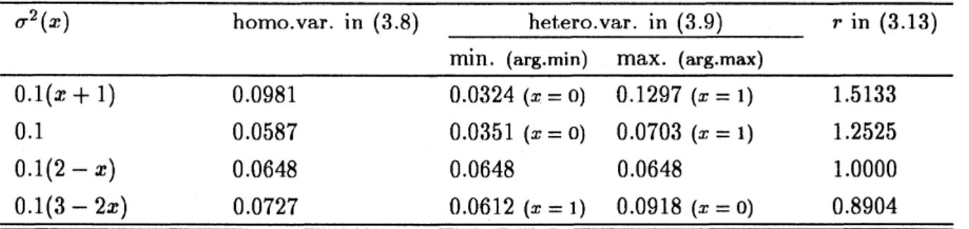
$r(f_{X}(x), \sigma^{2}(x), m(x))=\frac{AMISE(m(x),\overline{m_{h_{VS}}}(x))}{AMISE(m(x),\overline{m_{h_{f*xed}}.}(x))}$, (3.13)

by the four types of conditional variance functions, $\sigma^{2}(x)=0.1(x+1),$ $0.1$,

0.1$(2-x)$ and 0.1$(3-2x)$. We show in Table 2 the asymptotic homoscedastic

variance in (3.8), the maximal and minimal values of the asymptotic

het-eroscedastic varia,nce _{in (3.9), and the ratio of the two AMISE} $s$

.

We observe

the ratio $r$ moves from 1.5133 to 0.8904. The practical implication obtained

here is that VS bandwidth outperforms the fixed bandwidth in terms of

AMISE if the conditional va,riance $\sigma^{2}(x)$ diminishes as _$x$ increases under the

a,ssumption that the regression function $m(x)$ is a monotone increa,sing.

$\overline{\overline{0..\cdot 1(x+1)0..09811513301(3-2x)007270.8904\sigma^{2}(x)homo.var.in(3.8)r..in(3.13)0.1(2-x)0.064810000010.05871.2525\frac{hetero.var..\cdot.\cdot in(3.9)}{0.0612(x=1)00918(x=0)\min.(arg.\min)\max.(arg.\max_{=0.0351(x=0)00703(x1)})0.0324(x=0)01297(x=1)0.064800648}}}$

Table 2: The result of numerical calculation for illustrative example 1 in

Nishida and Kanazawa (2010).

Similarly, in the illustrative example 2 in Nisihida and Kanazawa (2010),

we investigated how fat-tailedness of the distribution of $X$’s affects the ratio

$r$ of the AMISE $s$ in (3.13). This is because we expect low density $f_{X}(x)$

at and near the boundaries of $I=[0,1]$ makes the proposed VS bandwidth

very wide, rendering the bias not to be ignora,ble. The main result from

the illustrative exa,mple 2 is that the $VS$ bandwidth is more serviceable than

On the other hand, in comparison with the MSE minimizing variable

bandwidth, it is proved by the H\"older $s$ inequality that the

MSE

minimizing

variable bandwidth always achieve smaller AMISE than the VS bandwidth,

$AM$$ISE(m(x),\overline{m_{h_{var}}}(x))\leq AMISE(m(x),\overline{m_{h_{VS}}}(x))$

.

3.1.3 Estimation of the

univariate

VS bandwidth

We show one estima,ting procedure of the univa,riate _VS ba,ndwidth. _{In view}

of (3.7), we estimate the univariate VS ba,ndwidth _{by the plug-in approach,}

$\overline{h_{VS}}(x)=\hat{h}_{0}\cdot\frac{\sigma^{\hat{2}}(x)}{\hat{f_{X}}(x)}$, (3.14)

where $f_{X}(x)$ and $\sigma^{2}(x)$ are nonparametrically estimated and the constant

term $h_{0}$ is estimated by cross-validation method a,s in Marron and H\"ardle

(1986). As a candidate for $\hat{f_{X}}(x)$, we employ kernel density estimator, where

$\hat{h_{f}}$ is chosen to minimize the least-squares cross-validation as in Rudemo

(1982) and Bowman (1984). The $\hat{h_{f}}$ so obtained is known asymptotically

equivalent to the

MISE

optimized bandwidth of $h_{f}$ as in Hall (1983). As a

candidate for $\sigma^{\hat{2}}(x)$, we employ the residual based estimator,

$\frac{\sum_{i=1}^{n}K(arrow)(Y_{i}-\overline{m_{h_{v}}}(X_{i}))^{2}}{\sum_{i=1}^{n}K(x_{h_{v}}^{-}arrow x)}$, (3.15)

as $|n,$ for instance, Fan and $Yao$ (1998).

However when $estima,ting\sigma^{2}(x)$, we generally need to estimate $m(x)$

be-forehand, which needs an estimator of $\sigma^{2}(x)be,forehand$ beca,use we are in

the variance-sta,bilizing setting. Hence an iterative method that enables us

$\sim(o)$

to estimate $\sigma^{2}(x)$ and $m(x)$ simultaneously, like $(\sigma^{2}$ $(x)arrow\hat{m}^{(0)}(x)arrow$

$\sim(1)$

$\sigma^{2}$ _{$(x)arrow\hat{m}^{(1)}(x)arrow\ldots),$} is required. The following is an idea of the

itera-tive estimating procedure.

$\bullet$ Obtain $\overline{Y}$

as an initial value and compute squared residuals $r^{2,(0)}(X_{i})=(Y_{i}-Y)^{2}-$,

$i=1,$ $\ldots,$$n$.

$\bullet$ Obtain bandwidth

$h_{v}^{(O)}$

that minimizes the cross-validation statistic,

$CV(h_{v}^{(0)})= \frac{1}{n}\sum_{i=1}^{n}(r^{2,(0)}(X_{i})_{-i,h_{v}^{(O)}}-\sigma^{\overline{2}}(X_{i}))^{2}$,

with respect to $h_{v}^{(O)}$, where

$\sigma^{\overline{2}}-i,h_{v}^{(o)}(X_{i})=\frac{\sum_{j=1;j\neq i}^{n}K(\frac{X_{j}-X_{1}}{h_{v}^{(0)}})r^{2,(O)}(X_{i})}{\sum_{j=1;j\neq i}^{n}K(\frac{X_{i}-X_{1}}{h_{v}^{(o)}})}$.

$arrow(O)$

The estimated bandwidth is $h_{v}$

.

Obtain nonparametric estimator ofconditional variance as

$\overline{\sigma_{\frac{2}{h_{v}}(0)}}(x)=\frac{\sum_{i=1}^{n}K(\frac{x-X_{i}}{\overline{h_{1J}}^{(0)}})r^{2,(0)}(X_{i})}{\sum_{i=1}^{n}K(\frac{x-X_{i}}{\overline{h_{1\prime}}^{(o)}})}$ .

Stage 2: Estimation of $h_{0}^{(t)}$.

$\sim(0)$

$\bullet$ Obtain bandwidth $h_{0}$ that minimizes the cross-validation statistic,

$CV( \hat{h_{0}}(0))=\frac{1}{n}\sum_{i=1}^{n}(Y_{i}-\hat{m}_{-i,h_{V9}^{-(o)(X_{i}))^{2}}}$,

$-(O)$

with respect to $h_{0}$ , where

$\hat{h_{VS^{()}}}(X_{i})=\frac{\overline{\sigma_{\frac{2}{h_{v}}(0)}}(X_{i})}{\hat{f_{h_{f}}}(X_{i})}\cdot\hat{h_{0}}io(0),=1,$

$\ldots,$$n$.

$\bullet$ Obtain NW type estimator $\overline{m_{h_{VS}^{-(0)}}}(X_{i})=\frac{\Sigma_{j--1}^{\mathfrak{n}}K(\frac{x.-x_{j}}{h\overline{\backslash r}q^{(0)}(X_{i})})Y_{j}}{\Sigma_{j=1}^{n}K(\frac{x_{1}-x_{j}}{h_{VS}^{-(0)}(X_{i})})},$ $i=1,$

$\ldots,$$n$.

$\bullet$ Compute squared residuals

$r^{2,(1)}(X_{i})=(Y_{i}-\overline{m_{h_{VS}^{-(o)}}}(X_{i}))^{2},$ $i=1,$ $\ldots,$$n$.

Stage 3

$\bullet$ Substitute

$r^{2,(O)}(X_{i})\wedge(t)$ in Stage 1 for $r^{2,(1)}(X_{i})$ in Stage 2 and repeat Stage 1 and

Output

We obtain $\hat{h_{v}}$

and $\hat{h_{0}}$

alternately.

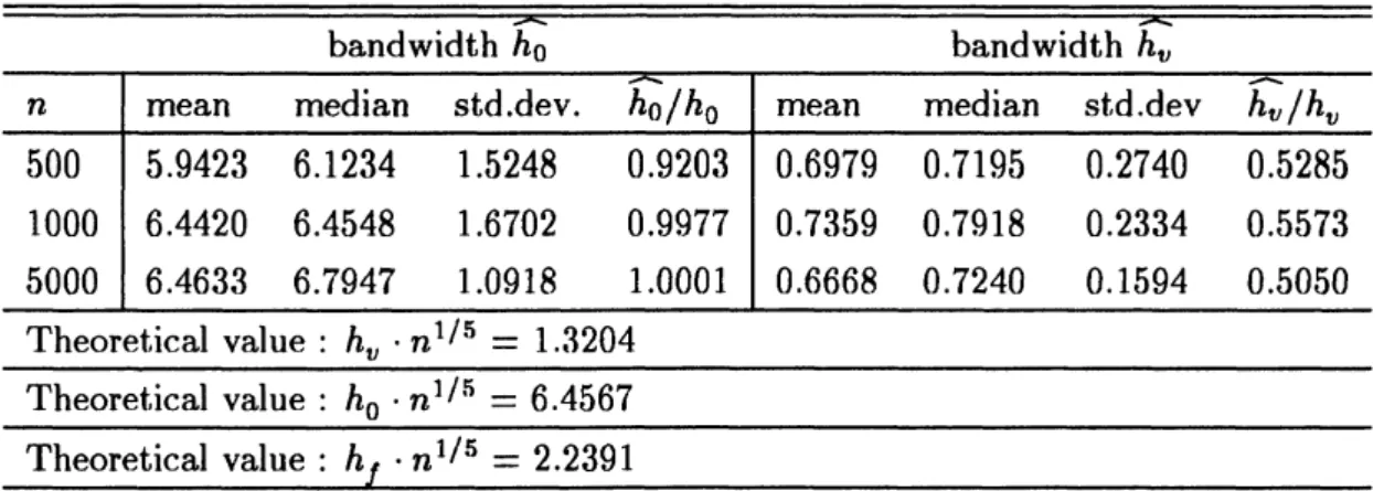
Simulation

We performed the simulation of the estimating procedure above. We

es-timated two bandwidths $\hat{h}_{v}$ and $\hat{h}_{0}$ by $N=50$ sets

of samplesize $n$ randomly

generated by the following functions $m(x)=0.5x^{2},$ $\sigma^{2}(x)=0.1(0.5|x|+0.1)$

and $fx(x)=N(0,4)\{x:-1<x<1\}$ on the domain [-1, 1]. In the

simula-tion, a data set is generated on $[-3.0,3.0]$ _{to eliminate boundary effect. The}

result and the plots of the estimated regression function are respectively on

Table 3 and Figure 1. The result on the table says that $\hat{h}_{0}$ is well estimated

while the estimation of $\hat{h_{v}}$ is poor. We

need further investigation on this

point.

$\overline{bandwidthh_{0}bandwidthh_{v}}$

Theoretical value: $h_{v}\cdot n^{1/5}=1.3204$

Theoretical value: $h_{0}\cdot n^{1/\backslash }=6.4567$

Theoretical value : $h_{f}\cdot n^{1/S}=2.2391$

Table 3: The result of the simulation. In the estimation, we employed

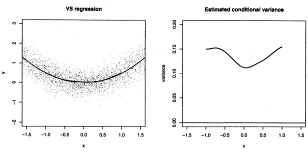
VS regression Estimated conditionalvarianco

$-1.5$ $-1.0$ $-0.5$ _{0.0 0.5 1.0 15} $-1.5$ $-1.0$ $-0.5$ 0.0 _{0.5 1.0 1.5}

xx

Figure 1: The left panel plots the va,ria,nce-stabilizing regression obta,ined _by

theestimating procedure. The right panel is the $nonparametric$ regression of

the conditional variance function obtained in the process of the estimating procedure.

3.2

Bivariate

VS

bandwidth

matrix:

$p=2$

When $p=2$, we can derive the optimal parameters $\eta_{0}^{*}(x)$ and $\eta_{1}^{*}(x)=$

$1-\eta_{0}^{*}(x)$ that minimize (3.6) at every $x$

.

The optimal $\eta_{0}^{*}(x)$ so obtained is

$\eta_{0}^{*}(x)=\{$

$\frac{\log[|\frac{o}{\alpha}\perp\Pi 3\mathfrak{c}|[\frac{\sigma^{2}(\mathfrak{c})}{f_{X}(\epsilon)}]^{2}]}{4\log[\frac{\sigma^{2}(\mathfrak{c})}{f_{X}(,\sigma)}]}$

, if $\alpha_{i}(x)\neq 0$, $i=1,2$,

(3.16)

any value satisfying $\eta_{0}^{*}(x)+\eta_{1}^{*}(x)=1$, if $\alpha_{i}(x)=0$, $i=1,2$

.

We give an interpreta,tion to the set of parameters $\eta_{i}(x),$ $i=1,2$

.

Com-pare the two terms (2.11) $and(3.4)$ that appear in the integrated squared

bia,$s$ terms. Since the term $[\sigma^{2}(x)/f_{X}(x)]^{2\eta i(x)}$ tha,t appears in (3.4) can be

considered as the penalty for the varia,nce _{stabilization, the para,meter} $\eta_{i}(x)$

stabi-lization between the axes. For example, if $\eta_{0}(x)=1/2$ and $\eta l(x)=1/2$, the

penalty for variance stabilization is equally distributed to each axis at the

point $x$

.

Similarly, if $\eta_{0}(x)=0$ and $\eta_{1}(x)=1$, all the penalty for variance

stabilization is incurred to the axis $x_{1}$ and no penalty is incurred to the $x_{0}$

axis at the point $x$ and vice versa.

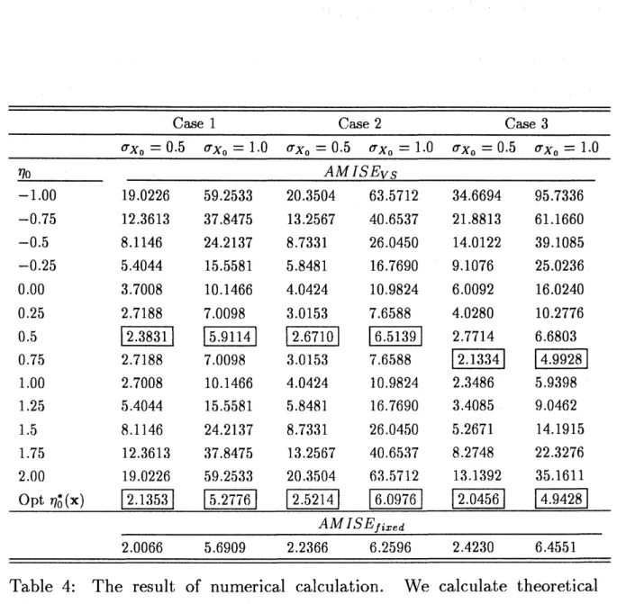
In the following, we arrangethenumerica,1 _{cases given} $m(x_{0}, x_{1}),$ $\sigma^{2}(x_{0}, x_{1})$

and $f_{X_{0},X_{1}}(x_{0}, x_{1})$, and calculate theoretica,1 AMISE $s$ by the different

band-width matrices. The one is calculated by the fixed bandwidth matrix in

(2.10) denoted by $AMISE_{fixed}$

.

The another is ca,lculated by the VS

band-width matrix in (3.3) denoted by $AMISE_{VS}$

.

As for the local parameters

$\eta_{i}(x)$ of the VS bandwidth matrix, we employ two types, the optimal one in

(3.16) and the universal one determined arbitrarily. The results a,re_on Table

4.

Casel: $m(x_{0},x_{1})=-3x_{0}^{2}-3x_{1}^{2},$$\sigma^{2}(x_{0},x_{1})=0.25,$ $f_{Xo,X_{1}}(x_{0},x_{1})\sim N(0,0,\sigma_{X_{0}},\sigma x_{1},P)$

trucated on $I^{2}=[-0.5,0.5]\cross[-0.5,0.5]$ and $\sigma_{X_{0}}=\sigma_{X_{1}},$ $\rho=0.0$

.

Case2: $m(x_{0}, x_{1})=-3x_{0}^{2}+2x_{0}x_{1}-3x_{1}^{2},$ $\sigma^{2}(x_{0}, x_{1})=0.25,$ $f_{X_{0},X_{1}}(x_{0}, x_{1})\sim$

$N(O, 0, \sigma_{X_{0}}, \sigma_{X_{1}}, \rho)$ trucated on $I^{2}=[-0.5,0.5]\cross[-0.5,0.5]$ and $\sigma_{X_{0}}=\sigma x_{1}$,

$\rho=0.0$

.

Case3: $m(x_{0}, x_{1})=\sin(2\pi x_{0})+x_{1},$ $\sigma^{2}(x_{0}, x_{1})=0.25,$ $f_{Xo,X_{1}}(x_{0}, x_{1})\sim$

$N(0,0, \sigma_{X_{0}}, \sigma_{X_{1}}, \rho)$ trucated on $I^{2}=[-0.5,0.5]\cross[-0.5,0.5]$ and $\sigma_{Xo}=\sigma_{X_{1}}$ ,

$\rho=0.0$

.

One main result obtained from the table is tha,$tAMISE_{VS}$ with optimal

loca,1 _para,meter, $\eta_{i}^{*}(x)$, is a,lways smaller than that with universal one

deter-mined arbitrarily. This result is a matter of course beca,use _{we optimized the}

local parameter so as to minimize AMISE. Another obtained result is that

$AMISE_{VS}$ can sometimes outperform $AMISE_{fixed}$

.

$Se_{\lrcorner}e$ the ca,ses 1,2 when

$\sigma_{X_{0}}=1$ and the case 3 when $\sigma_{X_{0}}=0.5,1$

.

In the case 3, we observe that

$AMISE_{VS}$ with universal local parameter can outperform $AMISE_{fixed}$

.

We

$\overline{\overline{CaselCase2Case3}}$

$\sigma_{X_{0}}=0.5$ $\sigma_{X_{0}}=1.0$ $\sigma_{X_{0}}=0.5$ $\sigma_{X_{0}}=1.0$ $\sigma_{X_{0}}=0.5$ $\sigma_{X_{0}}=1.0$

$\frac{\eta_{0}}{-1.00}$ $\frac{AMISE_{VS}}{59.253320.350463.571234.669495.7336}$ 19.0226 $-0.75$ 12.3613 37.8475 13.2567 40.6537 21.8813 61.1660 $-0.5$ 8.1146 24.2137 8.7331 26.0450 14.0122 39.1085 $-0.25$ 5.4044 15.5581 5.8481 16.7690 9.1076 25.0236 0.00 3.7008 10.1466 4.0424 10.9824 6.0092 16.0240 0.25 2.7188 7.0098 3.0153 7.6588 4.0280 10.2776 0.5 2.3831 $\frac{59114}{}$ 2.6710 6.5139 2.7714 6.6803 0.75 2.7188 7.0098 3.0153 7.6588 2.1334 4.9928 1.00 2.7008 10.1466 4.0424 IO.9824 2.3486 5.9398 1.25 5.4044 15.5581 5.8481 16.7690 3.4085 9.0462 1.5 8.1146 24.2137 8.7331 26.0450 5.2671 14.1915 1.75 12.3613 37.8475 13.2567 40.6537 8.2748 22.3276 2.00 19.0226 59.2533 20.3504 63.5712 13.1392 35.1611 $\frac{O_{P}t\eta_{0}^{*}(x)2.1_{*}3535.2776\frac{25214}{}-6.09762.04564.9428}{\frac{AMISE_{f.ixed}}{2.00665.69092.2366625962.42306.4551}}$

Table 4: The result of numerical ca,lculation. _{We calculate theoretical}

4

Concluding remark

In this paper, we limited the VS bandwidth matrix to the diagonal one by

the sphering approach and derived the theoretical form ofthe VS bandwidth

defined by two types of parameters $h_{0}$, global one, and $\eta_{i}(x)$, local one.

In the univariate case, we compared three bandwidths $h_{fixed},$ $h_{var}(x)$ and

$h_{VS}(x)$ in terms of local variance and AMISE. The implication obtained

here is that, in terms of local variance, $h_{VS}(x)$ can outperform both $h_{fixed}$

and $h_{var}(x)$ on some part of the domain. In terms of AMISE, $h_{VS}(x)$ can

sometimes outperform $h_{jixed}$, but never outperform $h_{var}(x)$

.

However, we observe a case where $h_{VS}(x)$ can be superior to the variable

bandwidth $h_{var}(x)$ in another point of view. At the point $x^{*}$ that satisfies

$\alpha^{2}(x^{*})=0$, the bandwidth $h_{var}(x^{*})$ takes infinitely large value. If $h_{var}(x^{*})$

approaches infinity, $\overline{m_{h_{ar}},,}(x^{*})$ a,pproaches to $\overline{Y}$

.

Then,

if $m(x^{*})$ does not

happen to agree with $\overline{Y},\overline{m_{h_{var}}}(x^{*})$ has unconformity at the point $x^{*}$

.

As for

$h_{vs}(x)$ in (3.7), such unconformity does not happen as long as $f_{X}(x)\neq 0$

.

If we consider this case, $VS$ bandwidth can be serviceable. Examples of

this kind of problem with variable bandwidth are illustrated in Nishida and

Kanawaza (2009) and can also be observed in the case of$p\geq 2$

.

In the bivariate case, we derived the optimal local parameters $\eta_{i}^{*}(x)$ and

give an interpretation. As a future study, we need to give further

investiga-tions to the bivariate case and develop a estimating procedure that can be

compared to the existing MSE based estimator as in Doksum (2000). We

also need to investigate the behavior of VS regression of$p\geq 3$

.

Appendix A

Suppose that the kernel function sa,tisfy:

K2 $\int\cdots\int tt^{T}K(t)dt<\infty$

.

K3 $\int\cdots\int K^{2}(t)dt<\infty$

.

K4 $\int\cdots\int|K(t)|dt<\infty$

.

$K5\lim_{tarrow\pm\infty}tK(t)arrow 0$

.

We place the following standa,rd _{set of assumptions:}

Al $H_{X}arrow 0$ as $n$ goes to infinity.

A2 $nH_{X}arrow\infty$ as $n$ goes to infinity.

A3 The density of X is $0<f_{X}(x)<\infty$ on a compa,ct support $I^{p}$

.

A4 The $f_{X}(x)$ is bounded continuously differentiable on $I^{p}$.

A5 The conditional va,ria,nce $\sigma^{2}(x)$ is continuous with respect to _$x$ and $0<$

$\sigma^{2}(x)<\infty$ on $I^{p}$

.

A6 The regression function $m(x)$ is twice bounded continuously

differen-tiable and is bounded and not identically constant on $I^{p}$

.

Appendix

$B$

We obtain the following relation between the two variances (3.9) and (3.10),

$AV_{X,Y}^{5}[\overline{m_{h_{var}}}(x)]-AV_{X,Y}^{5}[\overline{m_{h_{vs}}}(x)]$

$= \frac{[\int K^{2}(t)dt]^{4}}{[\int t^{2}K(t)dt]^{-2}}\frac{\int_{I^{1}}\frac{\sigma^{8}(x)\alpha^{2}(x)}{f_{X(x)}^{5}}d_{X}}{f_{X}(x)}[\frac{\frac{\sigma^{8}(x)\alpha^{2}(x)}{f_{X(x)}^{5}}}{\int_{I^{1}}\frac{\sigma^{8}(x)\alpha^{2}(x)}{f_{X}^{5}(x)}d_{X}}-f_{X}(x)]$ (B.1)

This is enough to show (3.11) because (B.1) is a subtraction of the twodensity

functions defined on the common domain $I^{1}$

.

References

Bowman, A, W. (1984). An alternative method ofcross-validation for the smoothing of

density estimates. Biometroka, 71, pp353-360.

Doksum, K., Peterson, D., Samarov, A. (2000). On variable bandwidth selection in local

Fan, J., Gijbels, I. (1992). Variable bandwidth and local linear regression smoothers.

Annals _ofstatistics, 20 (4), pp2008-2036.

Fan, J., Yao, Q. (1998). Efficient estimationofconditional variance functions in stochastic regression. Biomet$nka,$ $85(3)$, pp645-660.

Fukunaga, K. (1972). Introduction tostatistical pattern recognition. Academic press, New

York.

Hall, P. (1983). Large sample optimality ofleast square cross-validation in density

estima-tion. A nnals _ofstatistics, 11, pp1156-1174.

H\"ardle, W., M\"uller, M., Sperlich, S., Werwatz, A. (2004). Nonparametric and

Semipara-metric Models. Springer, Berlin and Heidelberg.

Marron, J.S., H\"ardle, W. (1986). Random approximations to some measures ofaccuracy

in nonparametric curve estimation. Journal _ofmultivariate Analysis, 20, pp91-113.

Nadaraya, E.A. (1964). On estimating regression. Theory_ofprobabilityandits applications,

9, pp141-142.

Nadaraya, E.A. (1965). On nonparametric estimation of density functions and regression

curves. Theory _ofprobability and its applications, 10, pp186-190.

Nadaraya, E.A. (1970). (Translated by B.Secklerfrom Russian) $R\epsilon$marks on

nonparamet-ric estimates for density functions and regression curves.Theory _ofprobability and its

applications, 15, pp134-137.

Nishida, K., and Kanazawa, J.Y. (2009). A note on the variance-stabilizing

nonparamet-ric regression. RIMS $K\hat{o}ky\hat{\iota}$_’roku, 1621, pp65-87. Research Institute for Mathematical

Sciences, Kyoto University, .lapan.

Nishida, K., and Kanazawa, J.Y. (2010). On variable variance-stabilizing bandwidth for

the Nadaraya-Watson regression estimator. Department _ofSocial $\iota 9ystems$ and

Manage-ment Discussion Paper Series, 1257, The Graduate School of Systemsand Information

Engineering, University ofTsukuba, Japan.

Rudemo, M. (1982). Empirical choice of histgrams and kernel densityestimators.

Scandi-navian Journol _ofStatistics, 9, pp65-78.

Wand, M.P., Jones, M.C. (1993). Comparison ofsmoothing parametrizations in bivariate

kernel density estimation. Journal _of the American Statistical Association, 88(422),

pp520-528.

Watson, G.S. (1964). Smooth regression analysis. Sankhya, Series $A,$ $26$, pp359-372.

Watson, G.S., Leadbetter, M.R. (1963). On theestimationof probability density, I. Annals